
 100% FREE ACCESS
12th Standard Syllabus & Materials
12th Standard
TN 12th Computer Applications மின்னணு தரவு பரிமாற்றம் Sample Question Papers Study Material - QB365 Set A
NEW12th Standard
TN 12th Computer Applications மின் - வணிக பாதுகாப்பு அமைப்புகள் Sample Question Papers Study Material - QB365 Set A
NEW12th Standard
TN 12th Computer Applications மின்னணு செலுத்தல் முறைகள் Sample Question Papers Study Material - QB365 Set A
NEW12th Standard
TN 12th Computer Applications மின் - வணிகம் Sample Question Papers Study Material - QB365 Set A
NEW12th Standard
TN 12th Computer Applications திறந்த மூல கருத்துருக்கள் Sample Question Papers Study Material - QB365 Set A
NEW12th Standard
TN 12th Computer Applications வலையமைப்பு வடமிடல் Sample Question Papers Study Material - QB365 Set A

Published on: 19/10/2019
Applied Statistics
Download Tamil Nadu 12th Standard Business Maths and Statistics question papers, model tests, one-mark questions, important questions, and public exam papers in PDF format. Free study materials and answer keys for TN State Board students.
Questions + Answers key
Take MCQ Business Maths and Statistics Test
1.
Define true value ratio.
2.
Write note on Fisher’s price index number.
3.
State the uses of Index Number.
4.
Define seasonal index.
5.
Define secular trend.
6.
State the uses of time series.
7.
Define Time series.
8.
Fit a trend line by the method of semi-averages for the given data.
| Year | 1990 | 1991 | 1992 | 1993 | 1994 | 1995 | 1996 | 1997 |
| Sales | 15 | 11 | 20 | 10 | 15 | 25 | 35 | 30 |
9.
State the different methods of measuring trend.
10.
A machine drills hole in a pipe with a mean diameter of 0.532 cm and a standard deviation of 0.002 cm. Calculate the control limits for mean of samples 5.
11.
Calculate four-yearly moving averages of number of students studying in a higher secondary school in a particular city from the following data.
| Year | 2001 | 2002 | 2003 | 2004 | 2005 | 2006 | 2007 | 2008 | 2009 |
| Sales | 124 | 120 | 135 | 140 | 145 | 158 | 162 | 170 | 175 |
12.
The following table shows the number of salesmen working for a certain concern:
| Year | 1992 | 1993 | 1994 | 1995 | 1996 |
| No. of salesmen | 46 | 48 | 42 | 56 | 52 |
Use the method of least squares to fit a straight line and estimate the number of salesmen in 1997.
13.
Determine the equation of a straight line which best fits the following data
| Year | 2000 | 2001 | 2002 | 2003 | 2004 |
| Sales(Rs.000) | 35 | 36 | 79 | 80 | 40 |
Compute the trend values for all years from 2000 to 2004
14.
The following data gives readings of 10 samples of size 6 each in the production of a certain product. Draw control chart for mean and range with its control limits.
| Sample | 1 | 2 | 3 | 4 | 5 | 6 | 7 | 8 | 9 | 10 |
| Mean | 383 | 508 | 505 | 582 | 557 | 337 | 514 | 614 | 707 | 753 |
| Range | 95 | 128 | 100 | 91 | 68 | 65 | 148 | 28 | 37 | 80 |
15.
16.
Calculate the cost of living index number for the year 2015 with respect to base year 2010 of the following data.
\(\begin{array}{|c|c|c|c|} \hline \text { Commodities } & \begin{array}{c} \text { Number of } \\ \text { Units (2010) } \end{array} & \begin{array}{c} \text { Price } \\ (2010) \end{array} & \begin{array}{c} \text { Price } \\ (2015) \end{array} \\ \hline \text { Rice } & 5 & 1500 & 1750 \\ \hline \text { Sugar } & 3.5 & 1100 & 1200 \\ \hline \text { Pulses } & 3 & 800 & 950 \\ \hline \text { Cloth } & 2 & 1200 & 1550 \\ \hline \text { Ghee } & 0.75 & 550 & 700 \\ \hline \text { Rent } & 12 & 2500 & 3000 \\ \hline \text { Fuel } & 8 & 750 & 600 \\ \hline \text { Misc } & 10 & 3200 & 3500 \\ \hline \end{array}\)
17.
the Laspeyre’s, Paasche’s and Fisher’s price index number for the following data. Interpret on the data.
| Commodities | Price | Quandity | ||
| 2000 | 2010 | 2000 | 2010 | |
| Rice | 38 | 35 | 6 | 7 |
| Wheat | 12 | 18 | 7 | 10 |
| Rent | 10 | 15 | 10 | 15 |
| Fuel | 25 | 30 | 12 | 16 |
| Miscellaneous | 30 | 33 | 8 | 10 |
18.
Given below are the data relating to the sales of a product in a district.
Fit a straight line trend by the method of least squares and tabulate the trend values.
| Year | 1995 | 1996 | 1997 | 1998 | 1999 | 2000 | 2001 | 2002 |
| Sales | 6.7 | 5.3 | 4.3 | 6.1 | 5.6 | 7.9 | 5.8 | 6.1 |
19.
The LCL for R chart is given by ________.
\({ D }_{ 2 }\bar { R } \)
\({ D }_{ 2 }\overset { = }{ R } \)
\({ D }_{ 3 }\overset { = }{ R } \)
\({ D }_{ 3 }\bar { R } \)
20.
R is calculated using ________.
xmax - xmin
xmin - xmax
\(\overset{-}{x}\)max - \(\overset{-}{x}\)min
\(\overset{=}{x}\)max - \(\overset{=}{x}\)min
21.
\(\overset {-}{X}\) chart is a ________.
attribute control chart
variable control chart
neither Attribute nor variable control chart
both Attribute and variable control chart
22.
The assignable causes can occur due to ________.
poor raw materials
unskilled labour
faulty machines
all of them
23.
How many causes of variation will affect the quality of a product?
4
3
2
1
24.
While computing a weighted index, the current period quantities are used in the: ________.
Laspeyre’s method
Paasche’s method
Marshall Edgeworth method
Fisher’s ideal method
25.
Laspeyre’s index = 110, Paasche’s index = 108, then Fisher’s Ideal index is equal to: ________.
110
108
100
109
26.
Another name of consumer’s price index number is: ________.
Whole-sale price index number
Cost of living index
Sensitive
Composite
27.
The value of ‘b’ in the trend line y = a + bx is ________.
Always positive
Always negative
Either positive or negative
Zero
28.
1.
The ratio between the total value of current period and total value of the base period is known as true value ratio.
(\( \frac{\sum P_{1} q_{1}}{\sum p_{0} q_{0}}\) is a true value tario)
2.
Fisher's price index number is the geometric mean of Laspeyre's and Paasche's price index number. Hence it is weighted index number.
Fisher's price index number = \(\sqrt {\frac {\sum p_{1}q_{0}}{\sum p_{0}q_{0} }}{\times}{\frac {\sum p_{1}q_{1}}{\sum p_{0}q_{1}} \times {100}}\)
3.
(i) It is an important tool for the formulating decision and management policies
(ii) It helps in studying the trends and tendencies
(iii) It determines the inflation and deflation in an economy
4.
Seasonal index is a measure of how a particular season compares with the average season.
5.
It is a general tendency of time series to increase or decrease or stagnates during a long period of time. An upward tendency is usually observed in population of a country, production, sales, prices in industries, income of individuals etc., A downward tendency is observed in deaths,epidemics, prices of electronic gadgets, water sources, mortality rate etc. It is not necessarily that the increase or decrease should be in the same direction throughout the given period of time. This feature is known as secular trend.
6.
Time series has an important objective to identify the variations and try to eliminate the variations and also helps us to estimate or predict the future values.
7.
A time series consists of a set of observations arranged in chronological order (either ascending or descending). It is a statistical data which relates to successive intervals or point of time.
8.
Since the number of years is even(eight), we can equally divide the given data it two equal parts and obtain the averages of first four years and last four years.
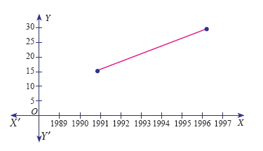
| Year | Production | Average |
| 1990 | 15 | \(\frac{15+11+20+10}{4}=14\) |
| 1991 | 11 | |
| 1992 | 20 | |
| 1993 | 10 | |
| 1994 | 15 | \(\frac{15+25+35+30}{4}=26.25\) |
| 1995 | 25 | |
| 1996 | 35 | |
| 1997 | 30 |
9.
The different methods of measurements of trends are
(i) Free hand or graphic method
(ii) Method of semi averages
(iii) Method of moving averages
(iv) Method of least squares
10.
Given \(\bar { X } \) = 0532., σ = 0.002, n = 5
The control limits for \(\overset{-} {X}\) chart is
\(UCL=\overset { = }{ X } +3\frac { \sigma }{ \sqrt { n } } =0.532+3\frac { 0.002 }{ \sqrt { 5 } } =0.5346\)
\(CL=\overset { = }{ X } =0.532\)
\(UCL=\overset { = }{ X } -3\frac { \sigma }{ \sqrt { n } } =0.532-3\frac { 0.002 }{ \sqrt { 5 } } =0.5293\)
11.
Computation of four- yearly moving averages.
| Year | Sales | 4-yearly centered moving total | 4-yearly moving Average | 4-yearly centered moving Average |
| 2001 | 124 | --- | -- | -- |
| 2002 | 120 | -- | -- | -- |
| 519 | 129.75 | |||
| 2003 | 135 | -- | 139.37 | |
| 540 | 135 | |||
| 2004 | 140 | -- | 139.75 | |
| 578 | 144.50 | |||
| 2005 | 145 | -- | 147.87 | |
| 605 | 151.25 | |||
| 2006 | 158 | -- | 162.50 | |
| 635 | 158.75 | |||
| 2007 | 162 | -- | 162.50 | |
| 665 | 166.25 | |||
| 2008 | 170 | -- | -- | - |
| 2009 | 175 | -- | -- | - |
12.
| Year (X) | No. of Salesmen Y | X = x -1994 | X2 | XY |
| 1992 | 46 | -2 | 4 | -92 |
| 1993 | 48 | -1 | 1 | -48 |
| 1994 | 42 | 0 | 0 | 0 |
| 1995 | 56 | 1 | 1 | 56 |
| 1996 | 52 | 2 | 4 | 104 |
| 244 | 0 | 10 | 20 |
Smce \(\sum\)X = 0, a =\(\frac {\sum Y}{n}\) = \(\frac {244}{5}\) = 48.8
b = \(\frac {\sum XY}{\sum X^2}\) = \(\frac {20}{10}\) = 2
∴ The required equation of the straight line trend is given by
Y = a + bX \(\Rightarrow \) Y = 48.8 + 2X
\(\Rightarrow \) Y = 48.8 +2 (X - 1994) .... (1)
∴ Number of salesmen in 1997 is put X = 1997 in (1)
∴ Y = 48.8 + 2 (1997 - 1994)
= 48.8 + 2 (3)
= 48.8 + 6 = 54.8
∴ Number of salesmen in 1997 is 54.8
13.
| Year | Sales | X=x- 2002 | X2 | XY |
| 2000 | 35 | -2 | 4 | -70 |
| 2001 | 36 | -1 | 1 | -36 |
| 2002 | 79 | 0 | 0 | 0 |
| 2003 | 80 | 1 | 1 | 80 |
| 2004 | 40 | 2 | 4 | 80 |
| 270 | 0 | 10 | 54 |
Since \(\sum X = 0, a = \frac{\sum Y}{n}\) = \(\frac {270}{5}\) = 54
b = \(\frac {\sum XY}{\sum X^2} = \frac {54}{10}\) = 5.4
∴ The required equation of the straight line trend is given by Y = a +bX
\(\Rightarrow \) Y = 54 + 5.4 (x - 2002)
The trend values can be obtained as follows:
When X = 2000, Yt = 54 + 5.4 (2000 - 2002)
= 54 + 5.4 (-2) = 43.2
When X = 2001, Yt = 54 + 5.4 (2001 - 2002)
= 54 + 5.4(-1) = 48.6
When X = 2002, Yt = 54 + 5.4 (2002 - 2002)
= 54
When X = 2003, Yt = 54 + 5.4 (2003 - 2002)
= 54 + 5.4 = 59.4
When X = 2004, Yt = 54 + 5.4 (2004 - 2002)
= 54 + 5.4 (2) = 64.8
14.
| Sample | 1 | 2 | 3 | 4 | 5 | 6 | 7 | 8 | 9 | 10 | Total |
| Mean | 383 | 508 | 505 | 582 | 557 | 337 | 514 | 614 | 707 | 753 | 5460 |
| Range | 95 | 128 | 100 | 91 | 68 | 65 | 148 | 28 | 37 | 80 | 840 |
\(\overset { = }{ X } =\frac { \sum { \bar { X } } }{ 10 } =\frac { 5460 }{ 10 } =546\)
The control limits for \(\overset{-}{X}\) chart is
\(UCL=\overset { = }{ X } +{ A }_{ 2 }\bar { R } =546+0.483(84)=586.57\)
\(CL=\overset { = }{ X } =546\)
\(LCL=\overset { = }{ X } -{ A }_{ 2 }\bar { R } =546-0.483(84)=505.43\)
\(\bar { R } =\frac { \sum { R } }{ n } =\frac { 840 }{ 10 } =84\)
The control limits for Range chart is
\(UCL={ D }_{ 4 }\bar { R } =2.004(84)=168.336\)
\(CL=\bar { R } =84\)
\(LCL={ D }_{ 3 }\bar { R } =0(84)=0\)
15.
16.
Here the base year quantities are given, therefore we can apply Aggregate Expenditure Method.
| Commodities | Number of Units q0(2010) |
Price (2010) p0 |
Price (2015) p1 |
p0q0 | p1q0 |
| Rice | 5 | 1500 | 1750 | 7500 | 8750 |
| Sugar | 3.5 | 1100 | 1200 | 3850 | 4200 |
| Pulses | 3 | 800 | 950 | 2400 | 2850 |
| Cloth | 2 | 1200 | 1550 | 2400 | 3100 |
| Ghee | 0.75 | 550 | 700 | 412.5 | 525 |
| Rent | 12 | 2500 | 3000 | 30000 | 36000 |
| Fuel | 8 | 750 | 600 | 6000 | 4800 |
| Misc | 110 | 3200 | 3500 | 32000 | 35000 |
| Total | 84562.5 | 95225 |
Cost of Living Index Number \(=\frac { \sum { { p }_{ 1 }{ q }_{ 0 } } }{ \sum { { p }_{ 0 }{ q }_{ 0 } } } \times 100=\frac { 95225 }{ 84562.5 } \times 100=112.609\)
Hence, the Cost of Living Index Number for a particular class of people for the year 2015 is increased by 12.61 % as compared to the year 2010.
17.
| Commodities | Price | Quandity | p0q0 | p0q1 | p1q0 | p1q1 | ||
| 2000 (p0) |
2010 q1 |
2000 (p0) |
2010 (q1) |
|||||
| Rice | 38 | 35 | 6 | 7 | 228 | 266 | 210 | 245 |
| Wheat | 12 | 18 | 7 | 10 | 84 | 120 | 126 | 180 |
| Rent | 10 | 15 | 10 | 15 | 100 | 150 | 150 | 225 |
| Fuel | 25 | 30 | 12 | 16 | 300 | 400 | 630 | 480 |
| Miscellaneous | 30 | 33 | 8 | 10 | 240 | 300 | 264 | 330 |
| Total | 952 | 1236 | 1110 | 1460 | ||||
Laspeyre’s price index number
\({ P }_{ 01 }^{ L }=\frac { \sum { { p }_{ 1 }{ q }_{ 0 } } }{ \sum { { p }_{ 0 }{ q }_{ 0 } } } \times 100=\frac { 1110 }{ 952 } \times 100=116.60\)
On an average, there is an increase of 16.60 % in the price of the commodities when the year 2000 compared with the year 2010.
Paasche’s price index number
\({ P }_{ 01 }^{ P }=\frac { \sum { { p }_{ 1 }{ q }_{ 1 } } }{ \sum { { p }_{ 0 }{ q }_{ 1 } } } \times 100=\frac { 1460 }{ 1236 } \times 100=118.12\)
On an average, there is an increase of 18.12 % in the price of the commodities when the year 2000 compared with the year 2010.
Fisher’s price index number
\({ P }_{ 01 }^{ F }=\sqrt { \frac { \sum { { p }_{ 1 }{ q }_{ 0 } } \times \sum { { p }_{ 1 }{ q }_{ 1 } } }{ \sum { { p }_{ 0 }{ q }_{ 0 } } \times \sum { { p }_{ 0 }{ q }_{ 1 } } } } \times 100=\sqrt { \frac { 1110\times 1460 }{ 952\times 1236 } } \times 100=117.36\)
On an average, there is an increase of 17.36 % in the price of the commodities when the year 2000 compared with the year 2010.
18.
Computation of trend values by the method of least squares.
In case of EVEN number of years, let us consider
\(X=\frac{\text{(x-Arithimetic mean of two middle years)}}{0.5}\)
| Year(x) | Sales(Y) | X=\(\frac{(x-1998.5)}{0.5}\) | XY | X2 | Trend Values (Yt) |
| 1995 | 6.7 | -7 | -46.9 | 49 | 5.6166 |
| 1996 | 5.3 | -5 | -26.5 | 25 | 5.7190 |
| 1997 | 4.3 | -3 | -12.9 | 9 | 5.8214 |
| 1998 | 6.1 | -1 | -6.1 | 1 | 5.9238 |
| 1999 | 5.6 | 1 | 5.6 | 1 | 6.0261 |
| 2000 | 7.9 | 3 | 23.7 | 9 | 6.1285 |
| 2001 | 5.8 | 5 | 29.0 | 25 | 6.2309 |
| 2002 | 6.1 | 7 | 42.7 | 49 | 6.3333 |
| N = 8 | 47.8 | \(\sum X\) = 0 | 8.6 | 168 |
\(a=\frac { \sum { Y } }{ n } =\frac { 47.8 }{ 8 } =5.975;\quad b=\frac { \sum { XY } }{ { \sum { X } }^{ 2 } } =\frac { 8.6 }{ 168 } =0.05119\)
Therefore, the required equation of the straight line trend is given by
Y = a + bX; Y = 5.975 + 0.05119 X.
When X = 1995, Yt = 5.975 + 0.05119\(\left( \frac { 1995-1998.5 }{ 0.5 } \right) =5.6166\)
When X = 1996, Yt = 5.975 + 0.05119\(\left( \frac { 1996-1998.5 }{ 0.5 } \right) =5.7190\)
similarly other values can be obtained.
19.
(d)
\({ D }_{ 3 }\bar { R } \)
20.
(a)
xmax - xmin
21.
(b)
variable control chart
22.
(d)
all of them
23.
(c)
2
24.
(b)
Paasche’s method
25.
(d)
109
26.
(b)
Cost of living index
27.
(c)
Either positive or negative
28.
(d)

12th Standard Syllabus & Materials
12th Standard
TN 12th Computer Applications களப்பெயர் முறைமை (DNS) Sample Question Papers Study Material - QB365 Set A
NEW12th Standard
TN 12th Computer Applications வலையமைப்பு எடுத்துக்காட்டுகள் மற்றும் நெறிமுறைகள் Sample Question Papers Study Material - QB365 Set A
NEW12th Standard
TN 12th Computer Applications கணினி வலையமைப்பு ஓர் அறிமுகம் Sample Question Papers Study Material - QB365 Set A
NEW12th Standard
TN 12th Computer Applications PHP-உடன் MySQL-ஐ இணைத்தல் Sample Question Papers Study Material - QB365 Set A



Tamilnadu Stateboard 12th Standard Subjects

Maths

Chemistry

Physics

Biology

Computer Science
Business Maths and Statistics

Economics

Commerce

Accountancy

History

Computer Applications
Biology
Computer Technology
Computer Applications
Computer Science
Business Maths and Statistics
Commerce
Economics
Maths
Chemistry
Physics
Computer Technology
History
Accountancy

Tamil

English

French
Tamilnadu Stateboard Standards
