
 100% FREE ACCESS
12th Standard Syllabus & Materials
12th Standard
TN 12th Maths Applications of Matrices and Determinants Sample Question Papers Study Material - QB365 Set A
NEW12th Standard
TN 12th Computer Applications மின்னணு தரவு பரிமாற்றம் Sample Question Papers Study Material - QB365 Set A
NEW12th Standard
TN 12th Computer Applications மின் - வணிக பாதுகாப்பு அமைப்புகள் Sample Question Papers Study Material - QB365 Set A
NEW12th Standard
TN 12th Computer Applications மின்னணு செலுத்தல் முறைகள் Sample Question Papers Study Material - QB365 Set A
NEW12th Standard
TN 12th Computer Applications மின் - வணிகம் Sample Question Papers Study Material - QB365 Set A
NEW12th Standard
TN 12th Computer Applications திறந்த மூல கருத்துருக்கள் Sample Question Papers Study Material - QB365 Set A

Published on: 01/10/2019
Applied Statistics
Download Tamil Nadu 12th Standard Business Maths and Statistics question papers, model tests, one-mark questions, important questions, and public exam papers in PDF format. Free study materials and answer keys for TN State Board students.
Questions + Answers key
Take MCQ Business Maths and Statistics Test
1.
Fit a trend line by the method of semi-averages for the given data.
| Year | 1990 | 1991 | 1992 | 1993 | 1994 | 1995 | 1996 | 1997 |
| Sales | 15 | 11 | 20 | 10 | 15 | 25 | 35 | 30 |
2.
3.
The following data gives the readings for 8 samples of size 6 each in the production of a certain product. Find the control limits using mean chart.
| Sample | 1 | 2 | 3 | 4 | 5 | 6 |
| Mean | 300 | 342 | 351 | 319 | 326 | 333 |
| Range | 25 | 37 | 20 | 28 | 30 | 22 |
Given for n = 6, A2 = 0.483,
4.
Fit a trend line by the method of semi-averages for the given data.
| Year | 2000 | 2001 | 2002 | 2003 | 2004 | 2005 | 2006 |
| Production | 105 | 115 | 120 | 100 | 110 | 125 | 135 |
5.
The following data gives readings of 10 samples of size 6 each in the production of a certain product. Draw control chart for mean and range with its control limits.
| Sample | 1 | 2 | 3 | 4 | 5 | 6 | 7 | 8 | 9 | 10 |
| Mean | 383 | 508 | 505 | 582 | 557 | 337 | 514 | 614 | 707 | 753 |
| Range | 95 | 128 | 100 | 91 | 68 | 65 | 148 | 28 | 37 | 80 |
6.
The data shows the sample mean and range for 10 samples for size 5 each. Find the control limits for mean chart and range chart.
| Sample | 1 | 2 | 3 | 4 | 5 | 6 | 7 | 8 | 9 | 10 |
| Mean | 21 | 26 | 23 | 18 | 19 | 15 | 14 | 20 | 16 | 10 |
| Range | 5 | 6 | 9 | 7 | 4 | 6 | 8 | 9 | 4 | 7 |
7.
Calculate the seasonal index for the quarterly production of a product using the method of simple averages.
| Year | I Quarter | II Quarter | III Quarter | IV Quarter |
| 2005 | 255 | 351 | 425 | 400 |
| 2006 | 269 | 310 | 396 | 410 |
| 2007 | 291 | 332 | 358 | 395 |
| 2008 | 198 | 289 | 310 | 357 |
| 2009 | 200 | 290 | 331 | 359 |
| 2010 | 250 | 300 | 350 | 400 |
8.
9.
Given below are the data relating to the sales of a product in a district.
Fit a straight line trend by the method of least squares and tabulate the trend values.
| Year | 1995 | 1996 | 1997 | 1998 | 1999 | 2000 | 2001 | 2002 |
| Sales | 6.7 | 5.3 | 4.3 | 6.1 | 5.6 | 7.9 | 5.8 | 6.1 |
10.
Given below are the data relating to the production of sugarcane in a district.
Fit a straight line trend by the method of least squares and tabulate the trend values.
| Year | 2000 | 2001 | 2002 | 2003 | 2004 | 2005 | 2006 |
| Prod.of Sugarcane | 40 | 45 | 46 | 42 | 47 | 50 | 46 |
1.
Since the number of years is even(eight), we can equally divide the given data it two equal parts and obtain the averages of first four years and last four years.
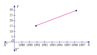
| Year | Production | Average |
| 1990 | 15 | \(\frac{15+11+20+10}{4}=14\) |
| 1991 | 11 | |
| 1992 | 20 | |
| 1993 | 10 | |
| 1994 | 15 | \(\frac{15+25+35+30}{4}=26.25\) |
| 1995 | 25 | |
| 1996 | 35 | |
| 1997 | 30 |
2.
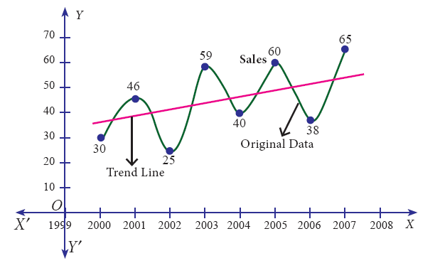
3.
| Sample | 1 | 2 | 3 | 4 | 5 | 6 | Total |
| Mean | 300 | 342 | 351 | 319 | 326 | 333 | 1971 |
| Range | 25 | 37 | 20 | 28 | 30 | 22 | 162 |
\(\overset { = }{ X } =\frac { \sum { \overset { - }{ X } } }{ number\ of\ samples } =\frac { 1971 }{ 6 } =328.5\quad \quad \overset { - }{ R } =\frac { \sum { R } }{ n } =\frac { 162 }{ 6 } =27\)
The control limits for \(\overset {-}{X}\) chart is
\(UCL=\overset { = }{ X } +{ A }_{ 2 }\overset { - }{ R } =328.5+0.483(27)=341.54\)
\(CL=\overset { = }{ X } =328.5\)
\(LCL=\overset { = }{ X } -{ A }_{ 2 }\overset { - }{ R } =328.5+0.483(27)=315.45\)
4.
Since the number of years is odd(seven), we will leave the middle year’s production value and obtain the averages of first three years and last three years.
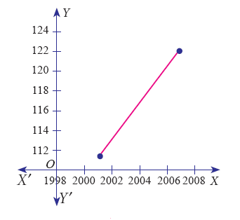
| Year | Production | Average |
| 2000 | 105 | \(\frac{105+115+120}{3}=113.33\) |
| 2001 | 115 | |
| 2002 | 120 | |
| 2003 | 100(left out) | |
| 2004 | 110 | \(\frac{110+125+135}{3}=123.33\) |
| 2005 | 125 | |
| 2006 | 135 |
5.
| Sample | 1 | 2 | 3 | 4 | 5 | 6 | 7 | 8 | 9 | 10 | Total |
| Mean | 383 | 508 | 505 | 582 | 557 | 337 | 514 | 614 | 707 | 753 | 5460 |
| Range | 95 | 128 | 100 | 91 | 68 | 65 | 148 | 28 | 37 | 80 | 840 |
\(\overset { = }{ X } =\frac { \sum { \bar { X } } }{ 10 } =\frac { 5460 }{ 10 } =546\)
The control limits for \(\overset{-}{X}\) chart is
\(UCL=\overset { = }{ X } +{ A }_{ 2 }\bar { R } =546+0.483(84)=586.57\)
\(CL=\overset { = }{ X } =546\)
\(LCL=\overset { = }{ X } -{ A }_{ 2 }\bar { R } =546-0.483(84)=505.43\)
\(\bar { R } =\frac { \sum { R } }{ n } =\frac { 840 }{ 10 } =84\)
The control limits for Range chart is
\(UCL={ D }_{ 4 }\bar { R } =2.004(84)=168.336\)
\(CL=\bar { R } =84\)
\(LCL={ D }_{ 3 }\bar { R } =0(84)=0\)
6.
| Sample | 1 | 2 | 3 | 4 | 5 | 6 | 7 | 8 | 9 | 10 | Total |
| Mean | 21 | 26 | 23 | 18 | 19 | 14 | 14 | 20 | 16 | 10 | 182 |
| Range | 5 | 6 | 9 | 7 | 4 | 6 | 8 | 9 | 4 | 7 | 65 |
\(\overset { = }{ X } =\frac { \sum { \overset { - }{ X } } }{ numberofsamples } =\frac { 182 }{ 10 } =18.2\quad \overset { - }{ R } =\frac { \sum { R } }{ n } =\frac { 65 }{ 10 } =6.5\)
The control limits for \(\overset{-}{X}\) chart is
\(UCL=\overset { = }{ X } +{ A }_{ 2 }\bar { R } =18.2+0.577(6.5)=21.95\)
\(CL=\overset { = }{ X } =18.2\)
\(LCL=\overset { = }{ X } -{ A }_{ 2 }\bar { R } =18.2-0.577(6.5)=14.5795\)
The control limits for Range chart is
\(UCL={ D }_{ 4 }\bar { R } =2.114(6.5)=13.741\)
\(CL=\bar { R } =65\)
\(LCL={ D }_{ 3 }\bar { R } =0(6.5)=0\)
7.
Computation of Seasonal Index by the method of simple averages.
| Year | I Quarter | II Quarter | III Quarter | IV Quarter |
| 2005 | 255 | 351 | 425 | 400 |
| 2006 | 269 | 310 | 396 | 410 |
| 2007 | 291 | 332 | 358 | 395 |
| 2008 | 198 | 289 | 310 | 357 |
| 2009 | 200 | 290 | 331 | 359 |
| 2010 | 250 | 300 | 350 | 400 |
| Quarterly Total |
1463 | 1872 | 2170 | 2321 |
| Quarterly Averages |
243.83 | 312 | 361.67 | 386.83 |
S.I for I Quarter = \(\frac{Average\ of \ I\ quarter }{Grand\ average} \times100\)
Grand Average = \(\frac{1304.333}{4}=326.0833\)
S.I for I Q = \(\frac{243.8333}{326.0833} \times100= 74.77;\)
S.I for II Q = \(\frac{312}{326.0833} \times100=95.68;\)
S.I for III Q = \(\frac{361.6667}{326.0833} \times 100=110.91; \)
S.I for IV Q = \(\frac{386.833}{326.0833} \times 100=118.63\)
8.
9.
Computation of trend values by the method of least squares.
In case of EVEN number of years, let us consider
\(X=\frac{\text{(x-Arithimetic mean of two middle years)}}{0.5}\)
| Year(x) | Sales(Y) | X=\(\frac{(x-1998.5)}{0.5}\) | XY | X2 | Trend Values (Yt) |
| 1995 | 6.7 | -7 | -46.9 | 49 | 5.6166 |
| 1996 | 5.3 | -5 | -26.5 | 25 | 5.7190 |
| 1997 | 4.3 | -3 | -12.9 | 9 | 5.8214 |
| 1998 | 6.1 | -1 | -6.1 | 1 | 5.9238 |
| 1999 | 5.6 | 1 | 5.6 | 1 | 6.0261 |
| 2000 | 7.9 | 3 | 23.7 | 9 | 6.1285 |
| 2001 | 5.8 | 5 | 29.0 | 25 | 6.2309 |
| 2002 | 6.1 | 7 | 42.7 | 49 | 6.3333 |
| N = 8 | 47.8 | \(\sum X\) = 0 | 8.6 | 168 |
\(a=\frac { \sum { Y } }{ n } =\frac { 47.8 }{ 8 } =5.975;\quad b=\frac { \sum { XY } }{ { \sum { X } }^{ 2 } } =\frac { 8.6 }{ 168 } =0.05119\)
Therefore, the required equation of the straight line trend is given by
Y = a + bX; Y = 5.975 + 0.05119 X.
When X = 1995, Yt = 5.975 + 0.05119\(\left( \frac { 1995-1998.5 }{ 0.5 } \right) =5.6166\)
When X = 1996, Yt = 5.975 + 0.05119\(\left( \frac { 1996-1998.5 }{ 0.5 } \right) =5.7190\)
similarly other values can be obtained.
10.
Computation of trend values by the method of least squares (ODD Years).
| Year(x) | Production of Sugarcane(Y) | X=(x–2003) | X2 | XY | Trend values(Yt) |
| 2000 | 40 | -3 | 9 | -120 | 42.04 |
| 2001 | 45 | -2 | 4 | -90 | 43.07 |
| 2002 | 46 | -1 | 1 | -46 | 44.11 |
| 2003 | 42 | 0 | 0 | 0 | 45.14 |
| 2004 | 47 | 1 | 1 | 47 | 46.18 |
| 2005 | 50 | 2 | 4 | 100 | 47.22 |
| 2006 | 46 | 3 | 9 | 138 | 48.25 |
| N=7 | \(\sum Y\)=316 | \(\sum X\)=0 | \(\sum X\)2=8 | \(\sum XY\)=29 | \(\sum Yt\)=316 |
\(a=\frac { \sum { Y } }{ n } =\frac { 316 }{ 7 } =45.143;\quad b=\frac { \sum { XY } }{ { \sum { X } }^{ 2 } } =\frac { 29 }{ 28 } =1.036\)
Therefore, the required equation of the straight line trend is given by
Y = a + bX
Y = 45.143 + 1.036 (x - 2003)
The trend values can be obtained by
When X = 2000 , Yt = 45.143 + 1.036(2000–2003) = 42.035
When X = 2001, Yt = 45.143 + 1.036(2001–2003) = 43.071,
similarly other values can be obtained.

12th Standard Syllabus & Materials
12th Standard
TN 12th Computer Applications வலையமைப்பு வடமிடல் Sample Question Papers Study Material - QB365 Set A
NEW12th Standard
TN 12th Computer Applications களப்பெயர் முறைமை (DNS) Sample Question Papers Study Material - QB365 Set A
NEW12th Standard
TN 12th Computer Applications வலையமைப்பு எடுத்துக்காட்டுகள் மற்றும் நெறிமுறைகள் Sample Question Papers Study Material - QB365 Set A
NEW12th Standard
TN 12th Computer Applications கணினி வலையமைப்பு ஓர் அறிமுகம் Sample Question Papers Study Material - QB365 Set A



Tamilnadu Stateboard 12th Standard Subjects

Maths

Chemistry

Physics

Biology

Computer Science
Business Maths and Statistics

Economics

Commerce

Accountancy

History

Computer Applications
Biology
Computer Technology
Computer Applications
Computer Science
Business Maths and Statistics
Commerce
Economics
Maths
Chemistry
Physics
Computer Technology
History
Accountancy

Tamil

English

French
Tamilnadu Stateboard Standards
