
 100% FREE ACCESS
12th Standard Syllabus & Materials
12th Standard
TN 12th Computer Applications மின்னணு தரவு பரிமாற்றம் Sample Question Papers Study Material - QB365 Set A
NEW12th Standard
TN 12th Computer Applications மின் - வணிக பாதுகாப்பு அமைப்புகள் Sample Question Papers Study Material - QB365 Set A
NEW12th Standard
TN 12th Computer Applications மின்னணு செலுத்தல் முறைகள் Sample Question Papers Study Material - QB365 Set A
NEW12th Standard
TN 12th Computer Applications மின் - வணிகம் Sample Question Papers Study Material - QB365 Set A
NEW12th Standard
TN 12th Computer Applications திறந்த மூல கருத்துருக்கள் Sample Question Papers Study Material - QB365 Set A
NEW12th Standard
TN 12th Computer Applications வலையமைப்பு வடமிடல் Sample Question Papers Study Material - QB365 Set A

Published on: 05/09/2019
Applied Statistics
Download Tamil Nadu 12th Standard Business Maths and Statistics question papers, model tests, one-mark questions, important questions, and public exam papers in PDF format. Free study materials and answer keys for TN State Board students.
Questions + Answers key
Take MCQ Business Maths and Statistics Test
1.
Define seasonal index.
2.
Discuss about irregular variation
3.
Explain cyclic variations.
4.
Fit a trend line by the method of semi-averages for the given data.
| Year | 1990 | 1991 | 1992 | 1993 | 1994 | 1995 | 1996 | 1997 |
| Sales | 15 | 11 | 20 | 10 | 15 | 25 | 35 | 30 |
5.
Calculate Fisher’s price index number and show that it satisfies both Time Reversal Test and Factor Reversal Test for data given below.
| Commodities | Base Year | Current Year | ||
| Price | Quantity | Price | Quantity | |
| Rice | 10 | 5 | 11 | 6 |
| Wheat | 12 | 6 | 13 | 4 |
| Rent | 14 | 8 | 15 | 7 |
| Fuel | 16 | 9 | 17 | 8 |
| Transport | 18 | 7 | 19 | 5 |
| Miscellaneous | 20 | 4 | 21 | 3 |
6.
Construct the Laspeyre’s, Paasche’s and Fisher’s price index number for the following data. Comment on the result.
| Commodities | Base Year | Current Year | ||
| Price | Quantity | Price | Quantity | |
| Rice | 15 | 5 | 16 | 8 |
| Wheat | 10 | 6 | 18 | 9 |
| Rent | 8 | 7 | 15 | 8 |
| Fuel | 9 | 5 | 12 | 6 |
| Transport | 11 | 4 | 11 | 7 |
| Miscellaneous | 16 | 6 | 15 | 10 |
7.
Calculate the seasonal index for the quarterly production of a product using the method of simple averages.
| Year | I Quarter | II Quarter | III Quarter | IV Quarter |
| 2005 | 255 | 351 | 425 | 400 |
| 2006 | 269 | 310 | 396 | 410 |
| 2007 | 291 | 332 | 358 | 395 |
| 2008 | 198 | 289 | 310 | 357 |
| 2009 | 200 | 290 | 331 | 359 |
| 2010 | 250 | 300 | 350 | 400 |
8.
Given below are the data relating to the production of sugarcane in a district.
Fit a straight line trend by the method of least squares and tabulate the trend values.
| Year | 2000 | 2001 | 2002 | 2003 | 2004 | 2005 | 2006 |
| Prod.of Sugarcane | 40 | 45 | 46 | 42 | 47 | 50 | 46 |
9.
Which of the following Index number satisfy the time reversal test?
Laspeyre’s Index number
Paasche’s Index number
Fisher Index number
All of them
10.
Laspeyre’s index = 110, Paasche’s index = 108, then Fisher’s Ideal index is equal to: ________.
110
108
100
109
11.
The component of a time series attached to long term variation is trended as ________.
Cyclic variation
Secular variations
Irregular variation
Seasonal variations
12.
The value of ‘b’ in the trend line y = a + bx is ________.
Always positive
Always negative
Either positive or negative
Zero
13.
1.
Seasonal index is a measure of how a particular season compares with the average season.
2.
Irregular variations do not have particular pattern and there is no regular period of time of their occurrences. Normally they are short terms variations but its occurrence sometimes has its effect so intense that they may give rise to new cyclic or other movements of variations.
For example floods, wars, earthquakes, Tsunami, strikes, lockouts etc.
3.
Cyclic uniformly periodic in nature. They may or may not follow exactly similar patterns after equal intervals of time. Generally one cyclic period ranges from 7 to.9 years and there is no hard and fast rule in the fixation of years for a cyclic period. For example, every business cycle has a Start-Boom-Depression- Recover maintenance during booms and depressions, changes in government monetary policies, changes in interestrates.
4.
Since the number of years is even(eight), we can equally divide the given data it two equal parts and obtain the averages of first four years and last four years.
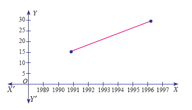
| Year | Production | Average |
| 1990 | 15 | \(\frac{15+11+20+10}{4}=14\) |
| 1991 | 11 | |
| 1992 | 20 | |
| 1993 | 10 | |
| 1994 | 15 | \(\frac{15+25+35+30}{4}=26.25\) |
| 1995 | 25 | |
| 1996 | 35 | |
| 1997 | 30 |
5.
| Commodities | Base Year | Current Year | p0q0 | p0q1 | p1q0 | p1q1 | ||
| Price (p0) |
Quantity (q1) |
Price ((p0)) |
Quantity (q1) |
|||||
| Rice | 10 | 5 | 11 | 6 | 50 | 60 | 55 | 66 |
| Wheat | 12 | 6 | 13 | 4 | 72 | 48 | 78 | 52 |
| Rent | 14 | 8 | 15 | 7 | 112 | 98 | 120 | 105 |
| Fuel | 16 | 9 | 17 | 8 | 144 | 128 | 153 | 136 |
| Transport | 18 | 7 | 19 | 5 | 126 | 90 | 133 | 95 |
| Miscellaneous | 20 | 4 | 21 | 3 | 80 | 60 | 84 | 63 |
| Total | 584 | 484 | 623 | 517 | ||||
Fisher’s price index number
\({ P }_{ 01 }^{ F }=\left( \sqrt { \frac { \sum { { p }_{ 1 }{ q }_{ 10 } } \times \sum { { p }_{ 1 }{ q }_{ 1 } } }{ \sum { { p }_{ 0 }{ q }_{ 0 } } \times \sum { { p }_{ 0 }{ q }_{ 1 } } } } \right) \times 100=\left( \sqrt { \frac { 623\times 517 }{ 584\times 484 } } \right) \times 100=106.74\)
Time Reversal Test: P01 × P10 = 1
\({ P }_{ 01 }\times { P }_{ 10 }=\sqrt { \left( \frac { \sum { { p }_{ 1 }{ q }_{ 0 } } \times \sum { { p }_{ 1 }{ q }_{ 1 } } \times \sum { { p }_{ 0 }{ q }_{ 1 } } \times \sum { { p }_{ 0 }{ q }_{ 0 } } }{ \sum { { p }_{ 0 }{ q }_{ 0 } } \times \sum { { p }_{ 0 }{ q }_{ 1 } } \times \sum { { p }_{ 1 }{ q }_{ 1 } } \times \sum { { p }_{ 1 }{ q }_{ 0 } } } \right) } \)
\({ P }_{ 01 }\times { P }_{ 10 }=\sqrt { \left( \frac { 623\times 517\times 484\times 584 }{ 584\times 487\times 517\times 623 } \right) } \)
P01 x P10 = 1
Factor Reversal Test
\({ P }_{ 01 }\times { Q }_{ 01 }=\frac { \sum { { p }_{ 1 }{ q }_{ 1 } } }{ \sum { { p }_{ 0 }{ q }_{ 0 } } } \)
\({ P }_{ 01 }\times { P }_{ 01 }=\sqrt { \left( \frac { \sum { { p }_{ 1 }{ q }_{ 0 } } \times \sum { { p }_{ 1 }{ q }_{ 1 } } \times \sum { { p }_{ 1 }{ q }_{ 0 } } \times \sum { { p }_{ 1 }{ q }_{ 1 } } }{ \sum { { p }_{ 0 }{ q }_{ 0 } } \times \sum { { p }_{ 0 }{ q }_{ 1 } } \times \sum { { p }_{ 0 }{ q }_{ 0 } } \times \sum { { p }_{ 0 }{ q }_{ 1 } } } \right) } \)
\({ P }_{ 01 }\times { P }_{ 10 }=\sqrt { \left( \frac { 623\times 517\times 484\times 517 }{ 584\times 484\times 584\times 623 } \right) } \)
\({ P }_{ 01 }\times { P }_{ 01 }=\sqrt { \left( \frac { 517\times 517 }{ 585\times 584 } \right) } =\frac { 517 }{ 584 } \)
\({ P }_{ 01 }\times { P }_{ 01 }=\frac { \sum { { p }_{ 1 }{ q }_{ 1 } } }{ \sum { { p }_{ 0 }{ q }_{ 0 } } } \)
6.
| Commodities | Base Year | Current Year | p0q0 | p0q1 | p1q0 | p1q1 | ||
| Price (p0) |
Quantity (q1) |
Price ((p0)) |
Quantity (q1) |
|||||
| Rice | 15 | 5 | 16 | 8 | 75 | 120 | 80 | 128 |
| Wheat | 10 | 6 | 18 | 9 | 60 | 90 | 108 | 162 |
| Rent | 8 | 7 | 15 | 8 | 56 | 64 | 105 | 120 |
| Fuel | 9 | 5 | 12 | 6 | 45 | 54 | 60 | 72 |
| Transport | 11 | 4 | 11 | 7 | 44 | 77 | 44 | 77 |
| Miscellaneous | 16 | 6 | 15 | 10 | 96 | 160 | 90 | 150 |
| Total | 376 | 565 | 487 | 709 | ||||
Laspeyre’s price index number
\({ P }_{ 01 }^{ L }=\frac { \sum { { p }_{ 1 }{ q }_{ 0 } } }{ \sum { { p }_{ 0 }{ q }_{ 0 } } } \times 100=\frac { 487}{ 376} \times 100=129.5212\)
Paasche’s price index number
\({ P }_{ 01 }^{ P }=\frac { \sum { { p }_{ 1 }{ q }_{ 1 } } }{ \sum { { p }_{ 0 }{ q }_{ 1 } } } \times 100=\frac { 709 }{ 565 } \times 100=125.4867\)
Fisher’s price index number
\({ P }_{ 01 }^{ F }=\sqrt { \frac { \sum { { p }_{ 1 }{ q }_{ 0 } } \times \sum { { p }_{ 1 }{ q }_{ 1 } } }{ \sum { { p }_{ 0 }{ q }_{ 0 } } \times \sum { { p }_{ 0 }{ q }_{ 1 } } } } \times 100=\sqrt { \frac { 487\times 709}{ 376\times 565} } \times 100=127.4879\)
On an average, there is an increase of 29.52%, 25.48% and 27.48% in the price of the commodities by Laspeyre’s, Paasche’s, Fisher’s price index number respectively, when the base year compared with the current year.
7.
Computation of Seasonal Index by the method of simple averages.
| Year | I Quarter | II Quarter | III Quarter | IV Quarter |
| 2005 | 255 | 351 | 425 | 400 |
| 2006 | 269 | 310 | 396 | 410 |
| 2007 | 291 | 332 | 358 | 395 |
| 2008 | 198 | 289 | 310 | 357 |
| 2009 | 200 | 290 | 331 | 359 |
| 2010 | 250 | 300 | 350 | 400 |
| Quarterly Total |
1463 | 1872 | 2170 | 2321 |
| Quarterly Averages |
243.83 | 312 | 361.67 | 386.83 |
S.I for I Quarter = \(\frac{Average\ of \ I\ quarter }{Grand\ average} \times100\)
Grand Average = \(\frac{1304.333}{4}=326.0833\)
S.I for I Q = \(\frac{243.8333}{326.0833} \times100= 74.77;\)
S.I for II Q = \(\frac{312}{326.0833} \times100=95.68;\)
S.I for III Q = \(\frac{361.6667}{326.0833} \times 100=110.91; \)
S.I for IV Q = \(\frac{386.833}{326.0833} \times 100=118.63\)
8.
Computation of trend values by the method of least squares (ODD Years).
| Year(x) | Production of Sugarcane(Y) | X=(x–2003) | X2 | XY | Trend values(Yt) |
| 2000 | 40 | -3 | 9 | -120 | 42.04 |
| 2001 | 45 | -2 | 4 | -90 | 43.07 |
| 2002 | 46 | -1 | 1 | -46 | 44.11 |
| 2003 | 42 | 0 | 0 | 0 | 45.14 |
| 2004 | 47 | 1 | 1 | 47 | 46.18 |
| 2005 | 50 | 2 | 4 | 100 | 47.22 |
| 2006 | 46 | 3 | 9 | 138 | 48.25 |
| N=7 | \(\sum Y\)=316 | \(\sum X\)=0 | \(\sum X\)2=8 | \(\sum XY\)=29 | \(\sum Yt\)=316 |
\(a=\frac { \sum { Y } }{ n } =\frac { 316 }{ 7 } =45.143;\quad b=\frac { \sum { XY } }{ { \sum { X } }^{ 2 } } =\frac { 29 }{ 28 } =1.036\)
Therefore, the required equation of the straight line trend is given by
Y = a + bX
Y = 45.143 + 1.036 (x - 2003)
The trend values can be obtained by
When X = 2000 , Yt = 45.143 + 1.036(2000–2003) = 42.035
When X = 2001, Yt = 45.143 + 1.036(2001–2003) = 43.071,
similarly other values can be obtained.
9.
(c)
Fisher Index number
10.
(d)
109
11.
(b)
Secular variations
12.
(c)
Either positive or negative
13.
(d)

12th Standard Syllabus & Materials
12th Standard
TN 12th Computer Applications களப்பெயர் முறைமை (DNS) Sample Question Papers Study Material - QB365 Set A
NEW12th Standard
TN 12th Computer Applications வலையமைப்பு எடுத்துக்காட்டுகள் மற்றும் நெறிமுறைகள் Sample Question Papers Study Material - QB365 Set A
NEW12th Standard
TN 12th Computer Applications கணினி வலையமைப்பு ஓர் அறிமுகம் Sample Question Papers Study Material - QB365 Set A
NEW12th Standard
TN 12th Computer Applications PHP-உடன் MySQL-ஐ இணைத்தல் Sample Question Papers Study Material - QB365 Set A



Tamilnadu Stateboard 12th Standard Subjects

Maths

Chemistry

Physics

Biology

Computer Science
Business Maths and Statistics

Economics

Commerce

Accountancy

History

Computer Applications
Biology
Computer Technology
Computer Applications
Computer Science
Business Maths and Statistics
Commerce
Economics
Maths
Chemistry
Physics
Computer Technology
History
Accountancy

Tamil

English

French
Tamilnadu Stateboard Standards
