
 100% FREE ACCESS
12th Standard Syllabus & Materials
12th Standard
TN 12th Computer Applications மின்னணு தரவு பரிமாற்றம் Sample Question Papers Study Material - QB365 Set A
NEW12th Standard
TN 12th Computer Applications மின் - வணிக பாதுகாப்பு அமைப்புகள் Sample Question Papers Study Material - QB365 Set A
NEW12th Standard
TN 12th Computer Applications மின்னணு செலுத்தல் முறைகள் Sample Question Papers Study Material - QB365 Set A
NEW12th Standard
TN 12th Computer Applications மின் - வணிகம் Sample Question Papers Study Material - QB365 Set A
NEW12th Standard
TN 12th Computer Applications திறந்த மூல கருத்துருக்கள் Sample Question Papers Study Material - QB365 Set A
NEW12th Standard
TN 12th Computer Applications வலையமைப்பு வடமிடல் Sample Question Papers Study Material - QB365 Set A

Published on: 09/03/2020
12th Standard Business Mathamatics English Medium All Chapter Book Back and Creative Five Marks Questions 2020
Download Tamil Nadu 12th Standard Business Maths and Statistics question papers, model tests, one-mark questions, important questions, and public exam papers in PDF format. Free study materials and answer keys for TN State Board students.
Questions + Answers key
Take MCQ Business Maths and Statistics Test
1.
From the data given below, calculate seasonal indices.
| Quarter | Year | ||||
| 1984 | 1985 | 1986 | 1987 | 1988 | |
| I | 40 | 42 | 41 | 45 | 44 |
| II | 35 | 37 | 35 | 36 | 38 |
| III | 38 | 39 | 38 | 36 | 38 |
| IV | 40 | 38 | 40 | 41 | 42 |
2.
Fit a straight line trend to the following data using the method of least square. Estimate the trend for 2007.
| year | 2000 | 2001 | 2002 | 2003 | 2004 |
| Sales (in tonnes) | 1 | 1.8 | 3.3 | 4.5 | 6.3 |
3.
A sample poll of 100 voters chosen at random from all voters in a given district indicated that 55% of them were in favour of a particular candidate. Find
(a) 95% confidence limits
(b) 99% confidence limits for the proportion to all voters in favour of this candidate.
4.
Measurements of the weights of a random sample of 200 ball bearings made by certain machine during one week showed a mean of 0.824 newtons and a S.D. of 0.042 newton's. Find
a) 95% and
b) 99% confidence limits for the mean weight of all the ball bearings.
5.
Marks in an aptitude test given to 800 students of a school was found to be normally distributed 10% of the students scored below 40 marks and 10% of the students scored above 90 marks. Find the number of students scored between 40 and 90?
6.
20% of the bolts produced in a factory are found to be defective. Find the probability that in a sample of 10 bolts chosen at random exactly 2 will be defective using
(i) Binomial distribution
(ii) Poisson distribution (e-2 = 0.1353)
7.
Solve the following assignment problem.
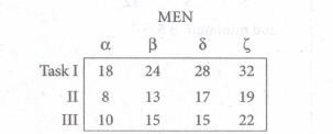
8.
Consider the problem of assigning five jobs to five persons. The assignment costs are given as follows. Determine the optimum assignment.
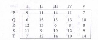
9.
The probability distribution of a random variable X is
| X | 1 | 2 | 4 | 2A | 3A | 5A |
| P(X) | \(\frac{1}{2}\) | \(\frac{1}{5}\) | \(\frac{3}{25}\) | \(\frac{1}{10}\) | \(\frac{1}{25}\) | \(\frac{1}{25}\) |
Calculate
(i) A if E(X) = 2.94
(ii) V(X)
10.
A discrete random variable X has the following probability distribution.
| x | 1 | 2 | 3 | 4 | 5 | 6 | 7 |
| P(X) | c | 2c | 2c | 3c | c2 | 2c2 | 7c2+c |
Find the value of e. Also, find the mean of the distribution.
11.
Using integrals as limit of sums, evaluate \(\int _{ 2 }^{ 4 }{ (2x-1) } dx\)
12.
Evaluate \(\int { \frac { 1 }{ { 3x }^{ 2 }+13x-10 } } dx\)
13.
Equipment maintenance and operating costs (are related to the overhaul interval x by the equation \({ x }^{ 2 }\frac { dc }{ dx } -10xc=-10\) with c = c0 and x = x0. Find c as a function of x.
14.
Solve: x2\(\frac { dy }{ dx } \) = y2+2xy given that y = 1, when x = 1
15.
From the following table, estimate the premium for a policy maturing at the age of 58.
| Age (x) | 40 | 45 | 50 | 55 | 60 |
| Premium (y) | 114.84 | 96.16 | 83.32 | 74.48 | 68.48 |
16.
From the following data, calculate the value of e1.75
| x | 1.7 | 1.8 | 1.9 | 2.0 | 2.1 |
| ex | 5.474 | 6.050 | 6.686 | 7.386 | 8.166 |
17.
The marginal cost C' (x) and marginal revenue R' (x) are given by C' (x) = 20 +\(\frac{x}{20}\) and R' (x) = 30. The fixed cost is Rs.200. Determine the maximum profit.
18.
A new transit system has just gone into operation in a city. Of those who use the transit system this year, 10% will switch over to using their own car next year and 90% will continue to use the transit system. Of those who use their cars this year, 80% will continue to use their cars next year and 20% will switch over to the transit system. Suppose the population of the city remains constant and that 50% of the commuters use the transit system and 50% of the commuters use their own car this year,
(i) What percent of commuters will be using the transit system after one year?
(ii) What percent of commuters will be using the transit system in the long run?
19.
The Marginal revenue for a commodity is MR=\(\frac { { e }^{ x } }{ 100 } +x+{ x }^{ 2 }\), find the revenue function.
20.
The sum of three numbers is 6. If we multiply the third number by 2 and add the first number to the result we get 7. By adding second and third numbers to three times the first number we get 12. Find the numbers using rank method
21.
Solve the following equation by using Cramer’s rule
2x + y −z = 3, x + y + z =1, x− 2y− 3z = 4
22.
Using Lagrange’s interpolation formula find a polynomial which passes through the points (0, –12), (1, 0), (3, 6) and (4,12).
23.
Using interpolation, find the value of f(x) when x = 15
| x | 3 | 7 | 11 | 19 |
| f(x) | 42 | 43 | 47 | 60 |
24.
Determine an initial basic feasible solution to the following transportation problem by using North West Corner rule
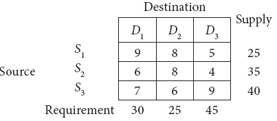
25.
A departmental head has four subordinates and four tasks to be performed. The subordinates differ in efficiency and the tasks differ in their intrinsic difficulty. His estimates of the time each man would take to perform each task is given below :
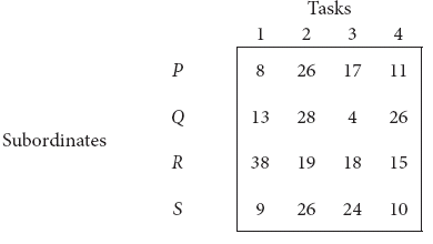
How should the tasks be allocated to subordinates so as to minimize the total man-hours?
26.
Solve \(\frac { dy }{ dx } +ycosx+x=2cosx\).
27.
The following are the sample means and ranges for 10 samples, each of size 5. Calculate the control limits for the mean chart and range chart and state whether the process is in control or not.
| Sample number | 1 | 2 | 3 | 4 | 5 | 6 | 7 | 8 | 9 | 10 |
| Mean | 5.10 | 4.98 | 5.02 | 4.96 | 4.96 | 5.04 | 4.94 | 4.92 | 4.92 | 4.98 |
| Range | 0.3 | 0.4 | 0.2 | 0.4 | 0.1 | 0.1 | 0.8 | 0.5 | 0.3 | 0.5 |
28.
A firm has found that the cost C of producing x tons of certain product by the equation x\(\frac { dC }{ dx } =\frac { 3 }{ x } -C\) and C = 2 when x = 1. Find the relationship between C and x.
29.
Calculate Fisher’s price index number and show that it satisfies both Time Reversal Test and Factor Reversal Test for data given below.
| Commodities | Price | Quandity | ||
| 2003 | 2009 | 2003 | 2009 | |
| Rice | 10 | 13 | 4 | 6 |
| Wheat | 125 | 18 | 7 | 8 |
| Rent | 25 | 29 | 5 | 9 |
| Fuel | 11 | 14 | 8 | 10 |
| Miscellaneous | 14 | 17 | 6 | 7 |
30.
The average score on a nationally administered aptitude test was 76 and the corresponding standard deviation was 8. In order to evaluate a state’s education system, the scores of 100 of the state’s students were randomly selected. These students had an average score of 72. Test at a significance level of 0.05 if there is a significant difference between the state scores and the national scores.
31.
A sample of 400 individuals is found to have a mean height of 67.47 inches. Can it be reasonably regarded as a sample from a large population with mean height of 67.39 inches and standard deviation 1.30 inches at 0.05 level of significance?
32.
The average daily sale of 550 branch offices was Rs.150 thousand and standard deviation is Rs. 15 thousand. Assuming the distribution to be normal, indicate how many branches have sales between
(i) Rs. 1,25,000 and Rs. 1, 45, 000
(ii) Rs. 1,40,000 and Rs. 1,60,000
33.
One fifth percent of the the blades produced by a blade manufacturing factory turn out to be defective. The blades are supplied in packets of 10. Use Poisson distribution to calculate the approximate number of packets containing no defective, one defective and two defective blades respectively in a consignment of 1,00,000 packets (e–0.2 =.9802)
34.
The probability density function of a continuous random variable X is
\(f(x)=\left\{\begin{array}{l} a+b x^{2}, 0 \leq x \leq 1 \\ 0, \text { otherwise } \end{array}\right.\)
where a and b are some constants. Find
(i) a and b if E(X)\(\frac{3}{5}\)
(ii) Var(X).
35.
Integrate the following with respect to x.
ex (1+ x) log(xex)
36.
The elasticity of demand with respect to price p for a commodity is \(\eta _{ d }=\frac { p+2{ p }^{ 2 } }{ 100-p-{ p }^{ 2 } } \).Find demand function where price is Rs. 5 and the demand is 70.
37.
The amount of bread (in hundreds of pounds) x that a certain bakery is able to sell in a day is found to be a numerical valued random phenomenon, with a probability function specified by the probability density function f(x) is given by
\(f(x)=\left\{\begin{array}{l} Ax,for \ 0≤x10 \\ A(20−x),for \ 10 ≤x< 20 \\ 0,\quad \quad \quad otherwise \end{array}\right.\)
(a) Find the value of A.
(b) What is the probability that the number of pounds of bread that will be sold tomorrow is
(i) More than 10 pounds,
(ii) Less than 10 pounds, and
(iii) Between 5 and 15 pounds?
38.
Using integration find the area of the circle whose center is at the origin and the radius is a units.
39.
Evaluate \(\int { { \left( \log x \right) }^{ 2 } } dx\)
40.
80% of students who do maths work during one study period, will do the maths work at the next study period. 30% of students who do english work during one study period, will do the english work at the next study period. Initially there were 60 students do maths work and 40 students do english work.
Calculate,
(i) The transition probability matrix
(ii) The number of students who do maths work, english work for the next subsequent 2 study periods.
1.
| Year | Quarters | |||
| I | II | III | IV | |
| 1984 | 40 | 35 | 38 | 40 |
| 1985 | 42 | 37 | 39 | 38 |
| 1986 | 41 | 35 | 38 | 40 |
| 1987 | 44 | 38 | 38 | 42 |
| 1988 | 44 | 38 | 38 | 42 |
| Total | 212 | 181 | 189 | 201 |
| Average | 42.4 | 36.2 | 37.8 | 40.2 |
Grand average = \(\frac{42.4+36.2+37.8+40.2}{4}\)
= 39.15
Seasonal Index (S.1) = \(\frac{Quarterlyaverage}{Grand average}\times 100\)
Hence,
S.1 or I quarter = \(\frac{42.4}{39.15}\times100=108.30\)
S.1 or II quarter = \(\frac{36.2}{39.15}\times100=92.54\)
S.1 or III quarter = \(\frac{37.8}{39.15}\times100=96.55\)
S.1 or IV quarter = \(\frac{40.2}{39.15}\times100=102.68\)
2.
| Year x | Sales y | X = x-2002 | XY | X2 |
| 2000 | 1 | -2 | -2 | 4 |
| 2001 | 1.8 | -1 | -1.8 | 1 |
| 2002 | 3.3 | 0 | 0 | 0 |
| 2003 | 4.5 | 1 | 4.5 | 1 |
| 2004 | 6.3 | 2 | 12.6 | 4 |
| 16.9 | 0 | 13.3 | 10 |
Let the required equation of the straight line trend is
y = a + bX
Since Σx = 0. \(a = \frac{\Sigma y}{x} = \frac{16.9}{5}\)
\(b = \frac{\Sigma xy}{\Sigma x^2} = \frac{13.3}{10} = 1.33\)
Hence, the straight line trend is
y = 3.38 + 1.33 (x - 2002)
∴ The trend for 2007 is
yt = 3.38 + 1.33 (2007 - 2002)
⇒ yt = 3.38 + 1.33 (5)
⇒ yt = 3.38 + 6.65
⇒ yt = 10.03
3.
Given p = \(\frac { 55 }{ 100 } \)
∴ q = \(\frac { 45 }{ 100 } \) and n = 100
Standard error = \(\sqrt { \frac { pq }{ n } } =\sqrt { \frac { \frac { 55 }{ 100 } \times \frac { 45 }{ 100 } }{ 100 } } \)
= 0.0497
(a) As the level of significance α = 0.05 \(Z_{ \frac { \alpha }{ 2 } }\) = 1.96
∴ 95% confidence limits for proportion is given by \(p-Z_{ \frac { \alpha }{ 2 } }(S.E)\le p\ge p+Z_{ \frac { \alpha }{ 2 } }(S.E)\)
⇒ 0.55 - (1.96) (0.0497) ≤ p ≤ 0.55 + (1.96) (0.0497)
⇒ 0.453 ≤ p ≤ 0.647
∴ 95% confidence interval for proportion is (0.45, 0.65)
(b) As the level of significance is α = 0.01, \(Z_{ \frac { \alpha }{ 2 } }\) = 2.58
∴ 99% confidence limits for proportion is given by \(p-Z_{ \frac { \alpha }{ 2 } }(S.E)\le p\ge p+Z_{ \frac { \alpha }{ 2 } }(S.E)\)
⇒ 0.55 - (2.58) (0.0497) ≤ p ≤ 0.55 + (2.58) (0.0497)
⇒ 0.422 ≤ p ≤ 0.678
Hence, 99% confidence interval for proportion is (0.42, 0.68).
4.
Given sample size n = 200
Sample mean \(\bar { x } \) = 0.824
Sample S.D. s = 0.042
Standard error = \(\frac { s }{ \sqrt { n } } =\frac { 0.042 }{ \sqrt { 200 } } \)
= \(\frac { 0.042 }{ 14.14 } \) = 0.00270
(a) As the level of significance is α = 0.05, \(Z_{ \frac { \alpha }{ 2 } }\) = 1.96
∴ 95% confidence limits for μ are given by \(\bar { x } -Z_{ \frac { \alpha }{ 2 } }(S.E)\le \mu \le \bar { x } +Z_{ \frac { \alpha }{ 2 } }(S.E)\)
⇒ 0.824 - (1.96) (0.00270) ≤ μ ≤ 0.824 + (1.96) (0.00270)
⇒ 0.824 - 0.00582 ≤ μ ≤ 0.824 + 0.00582
⇒ 0.818 ≤ μ ≤ 0.832
Hence, the 95% confidence limits for μ is (0.818,0.832)
(b) As the level of significance is α =0.001, \(Z_{ \frac { \alpha }{ 2 } }\) = 2.58
∴ 99% confidence limits for μ are given by \(\bar { x } -Z_{ \frac { \alpha }{ 2 } }(S.E)\le \mu \le \bar { x } +Z_{ \frac { \alpha }{ 2 } }(S.E)\)
⇒ 0.824 - (2.58) (0.00270) ≤ μ ≤ 0.824 + (2.58) (0.00270)
⇒ 0.824 - 0.00582 ≤ μ ≤ 0.824 + 0.005825
⇒ 0.816 ≤ μ ≤ 0.832
Hence, the 99% confidence limits for μ is (0.816, 0.832)
5.
Let X denote the height of the student
Given P (X < 40) = 10% = \(\frac { 10 }{ 100 } \) =0.1
P(X> 90) = 10% = \(\frac { 10 }{ 100 } \) =0.1
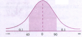
∴ P(40 < X < 90) = P(-∞ < X < ∞) - [P(X < 40) + P(X < 90)]
= 1 - (0.1 + 0.1)
= 1 - 0.2 = 0.8
∴ out of 800 students, number of students scored between 40 and 90 = 800 x 0.8
= 640 students.
6.
Given n = 10, p = \(\frac { 20 }{ 100 } =\frac { 1 }{ 5 } \)
∴ q = 1-p = \(1-\frac { 1 }{ 5 } =\frac { 4 }{ 5 } \)
Let
X denote the number of defective bolts chosen
∴ X = 2
(i) Using binomial distribution
P(X = 2) = \(10{ C }_{ 2 }\left( \frac { 1 }{ 5 } \right) ^{ 2 }\left( \frac { 4 }{ 5 } \right) ^{ 8 }\)
= \(\frac { 10\times 9 }{ 2\times 1 } \left( \frac { { 4 }^{ 8 } }{ { 5 }^{ 10 } } \right) =45\left( \frac { 4^{ 8 } }{ { 5 }^{ 10 } } \right) \)
(ii) Using Poisson distribution
λ = np = 10 \(\times\) \(\frac { 1 }{ 5 } \) = 2
P(X = x) \(\times\)\(\frac { { e }^{ -\lambda }.{ \lambda }^{ 0 } }{ x! } \)
x = 0,1,2,......n
∴ P(X = 2) = \(\frac { e^{ -2 }(2^{ 2 }) }{ 2 } =e^{ -2 }\left( \frac { 4 }{ 2 } \right) \)
= 2e-2
= 2(0.1353) = 0.2706
∴ P(X = 2) = 0.2706
7.
Since the number of rows is less then the number of columns, given assignment problem is unbalanced one.
To balance it, introduce a dummy row with all the entries zero.
The revised assignment problem is
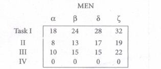
Here only 3 tasks can be assigned to 3 men.
Step 1 :
Select the smallest element in each row and subtract it will all the elements in its row.
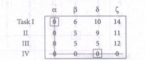
Here each row and column has atleast one zero.
Step 2:
Examine the row with only one zero, mark that zero by \(\Box\) and draw a vertical line.
After examining all the rows, examine the column with single zero, mark that zero by \(\Box\) and draw a horizontal line.
Step 3:
Only two assignment have been made.
The elements not lying on the line are
\(\begin{matrix} 6 & 10 & 14 \\ 5 & 9 & 11 \\ 5 & 5 & 12 \end{matrix}\)
and minimum is 5.
Subtract 5 from all these numbers. Other numbers remains the same.
A new cost matrix will be found .and repeat step 2.
∴ The new cost matrix is
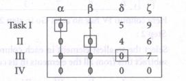
Thus, 3 assignments have been made.
The optical assignment schedule and total cost is
| Task | MEN | Cost |
| I | α | 18 |
| II | β | 13 |
| III | δ | 15 |
| Total Cost | Rs. 46 | |
8.
Here the number of rows and columns are equal.
∴ The given assignment problem is balanced.
Step 1 :
Select a smallest element in each row and subtract this from all the elements in its row.
∴ The cost matrix of the given assignment problem is
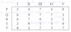
Here column IV has no zero. Go to step 2.
Step 2:
Select the smallest element in each column and subtract this from all the elements in its column.
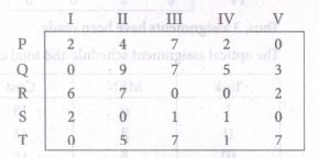
Since each row and column contains atleast one zero, assignments can be made.
Step 3:
Examine the row with exactly one zero. Mark the zero by \(\Box \) and draw a vertical line. After examining all the rows examine the column with one zero. mark the zero by \(\Box\) and draw a horizontal line.
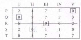
Here only 4 assignments have been made.
The numbers not lying on the line are
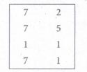
and min. of these numbers is 1.
Now subtract 1 from all these numbers and add 1 to the numbers on the intersecting line (ie. 6, 7, 2). Other numbers remains the same.
∴ The new cost matrix is
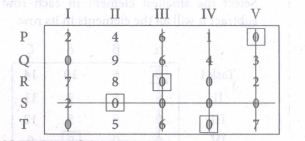
Now, repeat Step 3.
Thus, all the 5 assignments have been made.
The optimal assignment schedule and total cost is
| Person | Job | Cost |
| P | V | 7 |
| Q | I | 6 |
| R | III | 6 |
| S | II | 9 |
| T | IV | 10 |
| Total Cost | Rs. 38 | |
9.
E(X) = Σxi2pi
\(\Rightarrow E(X)=1(\frac { 1 }{ 2 } )+2\left( \frac { 1 }{ 5 } \right) +4\left( \frac { 3 }{ 25 } \right) +2A\left( \frac { 1 }{ 10 } \right) +3A\left( \frac { 1 }{ 25 } \right) +5A\left( \frac { 1 }{ 25 } \right) \)
\(\Rightarrow \frac { 1 }{ 2 } +\frac { 2 }{ 5 } +\frac { 12 }{ 25 } +\frac { A }{ 5 } +\frac { 3A }{ 25 } +\frac { A }{ 5 } \)
\(=\frac { 69 }{ 50 } +\frac { 13A }{ 25 } \)
Since E(X) = 2.94
\(\frac { 69 }{ 50 } +\frac { 13A }{ 25 } =2.94\Rightarrow \frac { 13A }{ 25 } =2.94-\frac { 69 }{ 50 } \)
= 2.94 - 1.38 = 1.56
\(\Rightarrow A=\frac { 1.56\times 25 }{ 13 } =\frac { 39 }{ 13 } =3\)
\(E({ X }^{ 2 })=1\left( \frac { 1 }{ 2 } \right) +4\left( \frac { 1 }{ 5 } \right) +16\left( \frac { 3 }{ 25 } \right) +{ (2A) }^{ 2 }\left( \frac { 1 }{ 10 } \right) { +(3A) }^{ 2 }\left( \frac { 1 }{ 25 } \right) +{ (5A) }^{ 2 }\left( \frac { 1 }{ 25 } \right) [\because A=3]\)
\(=\frac { 1 }{ 2 } +\frac { 4 }{ 5 } +\frac { 48 }{ 25 } +36\left( \frac { 1 }{ 10 } \right) \)
\(E({ X }^{ 2 })=\frac { 25+40+96+180+162+450 }{ 50 } \)
\(=\frac { 953 }{ 50 } =19.06\)
\(V(X)=E({ X }^{ 2 })-{ [E(X)] }^{ 2 }\)
\(=19.06-{ (2.94) }^{ 2 }[\because E(X)=2.94]\)
= 19.06 - 8.6436
V(X) = 10.4164
10.
Since X is the random variable taking values
1, 2,....7
P(X=1)+P(X=2)+...P(X=7) = 1
⇒ c+2c+2c+3c+c2+2c2+7c2+c = 1
⇒ 10c2+ 9c +1 = 0
⇒ (c+1)(10c-1)= 0
⇒ c = \(\frac{1}{10}\)[∵ c-1 is not possible]
Now, E(X) = Σxipi
= 1(c) + 2(2c) + 3(2c) + 4(3c) + 5c2 + 12c2 + 7(7c2 + c)
= 66c2+ 30c = 66(\(\frac{1}{10}\))2 + 30(\(\frac{1}{10}\))
= \(\frac{66}{100}+3=\frac{366}{100}=3.66\)
∴ E(X) = 3.66
11.
Let I = \(\int _{ 2 }^{ 4 }{ (2x-1) } dx\)
Here a = 2, b = 4 ⇒ \(h=\frac { b-a }{ n } =\frac { 4-2 }{ n } =\frac { 2 }{ n } \)
Given f(x) = 2x - 1
\(f(a+rh)=f\left( 2+r.\frac { 2 }{ n } \right) \)
= \(2\left( 2+\frac { 2r }{ n } \right) -1\)
= \(4+\frac { 4r }{ n } -1=3+\frac { 4r }{ n } \)
\(\therefore f(a+rh)=3+\frac { 4r }{ n } \)
\(\therefore \int _{ 2 }^{ 4 }{ (2x-1) } =\lim _{ n\rightarrow \infty }{ \sum _{ r=1 }^{ n }{ \frac { 2 }{ n } } } \left( 3+\frac { 4r }{ n } \right) \)
= \(\lim _{ n\rightarrow \infty }{ \sum _{ r=1 }^{ n }{ \frac { 2 }{ n } } } \left( 3+\frac { 4r }{ n } \right) \)
= \(\lim _{ n\rightarrow \infty }{ \sum _{ r=1 }^{ n }{ \left( \frac { 6 }{ n } +\frac { 8r }{ { n }^{ 2 } } \right) } } \)
= \(\lim _{ n\rightarrow \infty }{ \left( \frac { 6 }{ n } .\sum _{ r=1 }^{ n }{ .1 } +\frac { 8 }{ { n }^{ 2 } } .\sum _{ r=1 }^{ n }{ r } \right) } \)
= \(\lim _{ n\rightarrow \infty }{ \left( \frac { 6 }{ n } .n+\frac { 8 }{ { n }^{ 2 } } .\frac { n(n+1) }{ 2 } \right) } \)
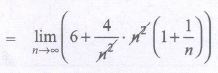
= \(6+4\lim _{ n\rightarrow \infty }{ \left( 1+\frac { 1 }{ n } \right) } \)
= \(\therefore \int _{ 2 }^{ 4 }{ (2x-1) } dx=10\)
= \(\left[ \because \sum _{ r=1 }^{ n }{ r } =n\& \sum _{ r=1 }^{ n }{ r } n=\frac { n(n+1) }{ 2 } \right] \)
12.
Let I = \(\int { \frac { 1 }{ { 3x }^{ 2 }+13x-10 } } dx\)
= \(\frac { 1 }{ 3 } \int { \frac { dx }{ { x }^{ 2 }+\frac { 13 }{ 3 } x-\frac { 10 }{ 3 } } } \)
= \(\frac { 1 }{ 3 } \int { \frac { dx }{ { x }^{ 2 }+\frac { 13 }{ 3 } x+\frac { 169 }{ 36 } -\frac { 169 }{ 36 } -\frac { 10 }{ 3 } } } \)
= \(\frac { 1 }{ 3 } \int { \frac { dx }{ { \left( x+\frac { 13 }{ 6 } \right) }^{ 2 }-\frac { 289 }{ 36 } } } \)
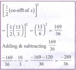
= \(\frac { 1 }{ 3 } \int { \frac { dx }{ { \left( x+\frac { 13 }{ 6 } \right) }^{ 2 }-{ \left( \frac { 17 }{ 16 } \right) }^{ 2 } } } \)
= \(\left[ \because \int { \frac { dx }{ { x }^{ 2 }-{ a }^{ 2 } } =\frac { 1 }{ 2a } log\left| \frac { x-a }{ x+a } \right| } +c \right] \)
= \(\frac { 1 }{ 3 } \times \frac { 1 }{ 2\times \frac { 17 }{ 6 } } log\left| \frac { x+\frac { 13 }{ 6 } -\frac { 17 }{ 6 } }{ x+\frac { 13 }{ 6 } +\frac { 17 }{ 6 } } \right| +c\)
= \(\frac { 1 }{ 17 } log\left| \frac { x-\frac { 2 }{ 5 } }{ x+5 } \right| +c\)
= \(\frac { 1 }{ 17 } log\left| \frac { 3x-2 }{ 3(x+5) } \right| +c\)
13.
\({ x }^{ 2 }\frac { dc }{ dx } -10xc=-10\)
\(\div { x }^{ 2 },\frac { dc }{ dx } -\frac { 10c }{ x } =\frac { 10 }{ { x }^{ 2 } } \frac { dc }{ dx } +Pc=Q\)
This is a first order linear differential equation of the form \(\frac{dc}{dx}\) + Pc = Q where
\(P=\frac { 10 }{ x }\) and \(Q=-\frac { 10 }{ { x }^{ 2 } } \)
\(\int { pdx } =-\int { \frac { 10 }{ x } =10logx=log\left( \frac { 1 }{ { x }^{ 10 } } \right) } \)
∴ I.F. = \({ e }^{ \int { pdf } }{ = }^{ { e }^{ log{ 1/x }^{ 10 } } }=\frac { 1 }{ { x }^{ 10 } } \)
∴ General solution is
\({ Ce }^{ \int { px } }=\int { Q.{ e }^{ \int { pdf } }dx+k } \)
\(\Rightarrow c.\left( \frac { 1 }{ { x }^{ 10 } } \right) =\int { -\frac { 10 }{ { x }^{ 2 } } . } \frac { 1 }{ { x }^{ 10 } } dx+k\)
\(=-10\int { \frac { 1 }{ { x }^{ 12 } } } dx+k\)
\(\Rightarrow \frac { c }{ { x }^{ 10 } } =-10\int { { x }^{ -12 } } dx+k\)
\(\Rightarrow \frac { c }{ { x }^{ 10 } } =\frac { 10 }{ 11 } \left( \frac { 1 }{ { x }^{ 11 } } \right) +k\)
\(\Rightarrow \frac { { C }_{ 0 } }{ { x }_{ 0 } } =\frac { 10 }{ 11 } \left( \frac { 1 }{ { x }_{ 0 }^{ 11 } } \right) +k\)
When c = c0, x = x0
\(\Rightarrow k=\frac { c }{ { x }_{ 0 }^{ 10 } } -\frac { 10 }{ 11.{ x }_{ 0 }^{ 11 } } \)
∴ The solution is
\(\Rightarrow \frac { c }{ x^{ 10 } } =\frac { 10 }{ 11 } \left( \frac { 1 }{ { x }^{ 11 } } \right) +k\left( \frac { c }{ { x }_{ 0 }^{ 10 } } -\frac { 10 }{ 11{ x }_{ 0 }^{ 11 } } \right) \)
\(\Rightarrow \frac { c }{ x^{ 10 } } -\frac { c }{ { x }_{ 0 }^{ 10 } } =\frac { 10 }{ 11 } \left( \frac { 1 }{ { x }^{ 11 } } -\frac { 10 }{ { x }_{ 0 }^{ 11 } } \right) \).
14.
Given x2\(\frac { dy }{ dx } \)= y2+2xy
⇒ \(\frac { dy }{ dx } =\frac { { y }^{ 2 }+2xy }{ x^{ 2 } } \)
The numerator and denominator are homogeneous function of degree
∴ put y = vx and \(\frac { dy }{ dx } =v+x\frac { dv }{ dx } \)
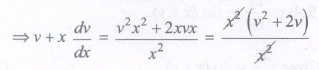
= v2+2v
⇒ v + x\(\frac { dv }{ dx } \) = v2+ 2v
⇒ x\(\frac { dv }{ dx } \) = v2+ 2v-v = v2+ v
Separating the variables,
\(\frac { dv }{ { v }^{ 2 }+v } =\frac { dx }{ x } \Rightarrow \frac { dv }{ v(v+1) } =\frac { dx }{ x } \)
[\(\frac { 1 }{ v(v+1) } =\frac { A }{ v } +\frac { B }{ v+1 } \)
1 = A(v+1)+Bv
put v = -1
1 = -B
put v = 0
1 = A
∴ \(\left( \frac { 1 }{ v } +\frac { 1 }{ v+v } \right) dv=\frac { dx }{ x } \)
Integrating
\(\int { \frac { dv }{ v } } -\int { \frac { dv }{ v+1 } } =\int { \frac { dx }{ x } } \)
⇒ log v - log (v + 1) - log x + log c
⇒ log\(\left( \frac { v }{ v+1 } \right) \)= log(xc)
⇒ \(\frac { v }{ v+1 } \)
Replacing v by \(\frac { y }{ x } \) we get,
\(\frac { \frac { y }{ x } }{ \frac { y }{ x } +1 } =xc\Rightarrow \frac { \frac { y }{ x } }{ \frac { x+y }{ x } } \) = xc
⇒ \(\frac { y }{ x+y } \) = xc
⇒ y = cx(x+y) ....(1)
Given, when x = -1, y = 1
∴ 1 = c(1) (1+1) ⇒ = 2c ⇒ c = \(\frac { 1 }{ 2 } \)
∴ (1) becomes, y = \(\frac { x }{ 2 } \)(x+y)
⇒ 2y = x(x+y)
15.
Using Newton's backward interpolation formula,
we can find y when x = 58.
∴ x + nh = x ⇒ 60 + n(5) = 58
⇒ 5n = 58 - 60 = -2
⇒ n = \(\frac{-2}{5}\)= -0.4
and y(58) = \({ y }_{ n }+\frac { n }{ n! } \nabla { y }_{ n }+\frac { n(n+1) }{ 2! } { \nabla }^{ 2 }{ y }_{ n }+\frac { n(n+1)(n-2) }{ 3! } { \nabla }^{ 3 }{ (y }_{ n })+\) .....
The difference table is
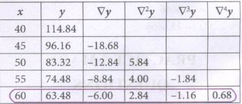
\(y(58)=68.48+\frac { (-0.4) }{ 1! } (-6)+\frac { (0.4)(-0.4+1) }{ 2! } (2.84)+\frac { (-0.4)(-0.4+1)(-0.4+2) }{ 3! } (-1.16)+\frac { (-0.4)(-0.4+2)(-0.4+2)(-0.4+3) }{ 3! } (0.68)\)
=68.48 + (0.4)(6) + \(\frac { (-0.4)(0.6) }{ 2 } (2.84)+\frac { (-0.4)(0.6)(1.6) }{ 6 } (-1.16)+\frac { (-0.4)(0.6)(1.6)(2.6) }{ 24 } (0.68)\)
= 68.48 + 2.4 - 0.3408 + 0.07424 - 0.028288
= 70.5851052
⇒ y(58) = 70.59
∴ Hence, premium for a policy maluting at the age of 58 is 70.59.
16.
Since e1.75 lies at the beginning of the table, we can use Newton's forward interpolation formula
∴ xo + nh = x ⇒ 1.7 + n(0.1) = 1.75
⇒ n(0.1) = 1.75 - 1.7 = 0.05
⇒ n = \(\frac{0.05}{0.1}\) = 0.5
\({ y }_{ x }={ y }_{ o }+\frac { n }{ n! } \triangle { y }_{ o }+\frac { n(n+1) }{ 2! } { \triangle }^{ 2 }{ y }_{ o }+\frac { n(n+1)(n-2) }{ 3! } { \triangle }^{ 3 }{ (y }_{ o })+.......\)
The difference table is
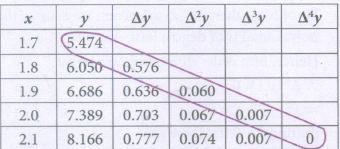
∴ \(y\left( { e }^{ 1.75 } \right) =5.74+\frac { 0.5 }{ 1! } (0.576)+\frac { (0.5)(0.5-1) }{ 2! } (0.06)+\frac { (0.5)(0.5-1)(0.5-2) }{ 3! } (0.007)\)
y(e1.75) = 5.474 + 0.288 - 0.0075 + 0.0004375
= 5.7549375
17.
Given \(C'(x)=20+\frac { x }{ 20 } \)
\(\Rightarrow \int { C'(x)dx= } \int { \left( 20+\frac { x }{ 20 } \right) dx } \)
\(C(x)=20x+\frac { { x }^{ 2 } }{ 40 } +{ k }_{ 1 }\)
Given when x = 0, C = 200
⇒ k1 = 200
\(\therefore C(x)=20x+\frac { { x }^{ 2 } }{ 40 } +200\quad ---(1)\)
Also, R'(x) = 30
\(R(x)=\int { 30dx } +{ k }_{ 2 }=30x+{ k }_{ 2 }\)
When x = 0 R = 0 ⇒ K2 = 0
∴ R(x) = 30x ----(2)
Profit = Total revenue - total cost
\(=30x-20x-\frac { { x }^{ 2 } }{ 40 } -200\)
\(\therefore P=10x-\frac { { x }^{ 2 } }{ 40 } -200---(3)\)
\(\frac { dp }{ dx } =10-\frac { 2x }{ 40 } =10-\frac { x }{ 20 } \)
\(\frac { dp }{ dx } =0\)
\(\Rightarrow 10-\frac { x }{ 20 } =0\)
\(\Rightarrow 10=\frac { x }{ 20 } \Rightarrow x=200\)
\(\frac { d^{ 2 }p }{ { dx }^{ 2 } } =-\frac { 1 }{ 20 } <0\)
∴ Profit is maximum when x= 200
∴ maximum profit \(P=10(200)-\frac { { (200) }^{ 2 } }{ 40 } -200[From(3)]\)
P = 2000 -1000 - 200
2000 - 1200
P = Rs .800.
Hence, the maximum profit is Rs. 800.
18.
Let A represents the percent of commuters who use the transit system and B represents the percent of commuters who use their own car. Transition probability matrix
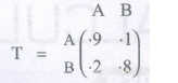
Given 50% of commuters use the transit system and 50% of the commuters use their own car this year.
(i) Percentage of commuters after one year
\(\left( \cdot 5\cdot 5 \right) \left( \begin{matrix} \cdot 9 & \cdot 1 \\ \cdot 2 & \cdot 8 \end{matrix} \right) \)
= (-5\(\times\)·9+·5\(\times\).2 ·5\(\times\)·1+·5\(\times\)·8)
= (-45 + ·10 ·05 +.40)
= (-55 - 45)
A = 55% and B = 45%
(ii) Equilibrium will be reached in the long run at equilibrium, we must have
(A B)T = (A B) wher A+B = 1
\(\Rightarrow \left( \begin{matrix} A & B \end{matrix} \right) \left( \begin{matrix} \cdot 9 & \cdot 1 \\ \cdot 2 & \cdot 8 \end{matrix} \right) =\left( \begin{matrix} A & B \end{matrix} \right) \)
\(\left( \begin{matrix} \cdot 9A+\cdot 2B & \cdot 1A+8B \end{matrix} \right) =\left( \begin{matrix} A & B \end{matrix} \right) \)
Equating the corresponding entries on both sides we get,
\(\cdot 9A+\cdot 2B=A\Rightarrow \cdot 9A+\cdot 2(1-A)=A\)
[Since A + B = 1, B = 1 -A]
\(\Rightarrow \cdot 9A+\cdot 2-\cdot 2A=A\)
\(\Rightarrow \cdot 2=A-\cdot 9A+\cdot 2A\)
\(\Rightarrow \cdot 2=A(1-\cdot 9+\cdot 2)\)
\(\Rightarrow \cdot 2=A=(\cdot 3)\)
\(\therefore\) 67% of the commuters will be using the transit system in the long run.
19.
Given that MR \(=\frac { { e }^{ x } }{ 100 } +x+{ x }^{ 2 }\)
\(\int { MR } =\int { \left( \frac { { e }^{ x } }{ 100 } +x+{ x }^{ 2 } \right) } dx\)
\(R=\frac { { e }^{ x } }{ 100 } +\frac { { x }^{ 2 } }{ 2 } +\frac { { x }^{ 3 } }{ 3 } +k\)
When x=0, R=0
\(\Rightarrow 0=\frac { { e }^{ 0 } }{ 100 } +0+0+k\)
\(k=-\frac { 1 }{ 100 } [\because { e }^{ 0 }=1]\)
∴ Revenue \(R=\frac { { e }^{ x } }{ 100 } +\frac { { x }^{ 2 } }{ 2 } +\frac { { x }^{ 3 } }{ 3 } +\frac { 1 }{ 100 } \)
20.
Let the three numbers be x, y and z respectively
Given
x + y + z = 6
x + 2z = 7
3x + y + z = 12
| Augmented matrix [A, B] |
Elementary Transformation' |
|---|---|
| \(\left( \begin{matrix} 1 & 1 & 1 \\ 1 & 0 & 2 \\ 3 & 1 & 1 \end{matrix}\begin{matrix} 6 \\ 7 \\ 12 \end{matrix} \right) \) | |
| \(\left( \begin{matrix} 1 & 1 & 1 \\ 0 & -1 & 1 \\ 0 & -2 & -2 \end{matrix}\begin{matrix} 6 \\ 1 \\ -6 \end{matrix} \right) \) | \({ R }_{ 2 }\rightarrow { R }_{ 2 }-{ R }_{ 1 }\) \({ R }_{ 3 }\rightarrow { R }_{ 2 }-3{ R }_{ 1 }\) |
| \(\sim \left( \begin{matrix} 1 & 1 & 1 \\ 0 & -1 & 1 \\ 0 & 0 & -4 \end{matrix}\begin{matrix} 6 \\ 1 \\ -8 \end{matrix} \right) \) | \({ R }_{ 3 }\rightarrow { R }_{ 3 }-2{ R }_{ 2 }\) |
The last equivalent matrix is in echelon form
\(\rho (A)=3\) and \(\rho (A,B)=3\)
\(\therefore \rho (A)=\rho (A,B)=3=Numberofunknowns\)
\(\therefore\) The system is consistent and has unique solution.
To find the solutions, let us rewrite the echelon form into matrix form
\(\left( \begin{matrix} 1 & 1 & 1 \\ 0 & -1 & 1 \\ 0 & 0 & -4 \end{matrix}\begin{matrix} x \\ y \\ z \end{matrix} \right) \left( \begin{matrix} x \\ y \\ z \end{matrix} \right) =\left( \begin{matrix} 6 \\ 1 \\ -8 \end{matrix} \right) \)
x + y + z = 6 ..(1)
-y + z = 1
-4z = -8
From (3),\(-4z=-8\Rightarrow z=\cfrac { -8 }{ -4 } =2\)
Substituting z = 2 in (2) we get
\(-y+2=1\Rightarrow -y=1-2\Rightarrow -y=-1\)
\(\Rightarrow y=1\)
Substitutingy = 1 andz = 2 in (1) we get
\(x+1+2=6\Rightarrow x+3=6\Rightarrow x=6-3\)
\(\Rightarrow x=3\)
Hence, the numbers are 3, 1, 2.
21.
\(\Delta =\left| \begin{matrix} 2 & 1 & -1 \\ 1 & 1 & 1 \\ 1 & -2 & 3 \end{matrix} \right| =2\)
\(\left| \begin{matrix} 1 & 1 \\ -2 & -3 \end{matrix} \right| -1\left| \begin{matrix} 1 & 1 \\ 1 & -3 \end{matrix} \right| -1\left| \begin{matrix} 1 & 1 \\ 1 & -2 \end{matrix} \right| \)
= 2 (-3+2) - 1 (-3 -1) -1 (-2-1)
= 2(-1) -1 (-4) -1 (-3)
= -2 + 4 + 3 = 5.
Since\(\Delta \neq 0\),
we can apply Cramer's rule and the system is consistent with unique solution.
\(x=\left| \begin{matrix} 3 & 1 & -1 \\ 1 & 1 & 1 \\ 4 & -2 & 3 \end{matrix} \right| =3\left| \begin{matrix} 1 & 1 \\ -2 & -3 \end{matrix} \right| -1\left| \begin{matrix} 1 & 1 \\ 4 & -3 \end{matrix} \right| -1\left| \begin{matrix} 1 & 1 \\ 4 & -2 \end{matrix} \right| \)
= 3(-3 + 2) -1(-3 -4) -1(-2 -4)
= 3 (-1) -1 (-7) -1 (-6)
= -3 + 7 + 6 = 10.
\(\Delta y=\left| \begin{matrix} 2 & 3 & -1 \\ 1 & 1 & 1 \\ 1 & 4 & -3 \end{matrix} \right| =2\left| \begin{matrix} 1 & 1 \\ 4 & -3 \end{matrix} \right| -3\left| \begin{matrix} 1 & 1 \\ 1 & -3 \end{matrix} \right| -1\left| \begin{matrix} 1 & 1 \\ 1 & 4 \end{matrix} \right| \)
= 2(-3 -4) -3 (-3 -1) -1 (4-1)
= 2 (-7) -3 (-4) -1(3)
= 14 + 12 - 3 = -5
\(\Delta z=\left| \begin{matrix} 2 & 1 & 3 \\ 1 & 1 & 1 \\ 1 & -2 & 4 \end{matrix} \right| \)
= \(2\left| \begin{matrix} 1 & 1 \\ -2 & 4 \end{matrix} \right| -1\left| \begin{matrix} 1 & 1 \\ 1 & 4 \end{matrix} \right| +3\left| \begin{matrix} 1 & 1 \\ 1 & -2 \end{matrix} \right| \)
= 2(4 + 2) -1(4 -1) + 3(-2 -1)
= 2(6) -1(3) + 3(-3)
= 12 - 3 - 9
= 0
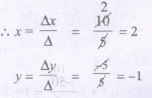
\(z=\cfrac { \Delta z }{ \Delta } =\cfrac { 0 }{ 5 } =0\)
\(\therefore\)Solution set is (2, -1, 0)
22.
Given
| x | 0 | 1 | 3 | 4 |
| y | -12 | 0 | 6 | 12 |
Here the intervals are unequal
∴ By Lagranges interpolation formula, we have
x0 = 0, x1 = 1, x2 = 3, x3 = 4
y0 = -12, y1 = 0, y2 = 6, y3 = 12 and x = x.
∴ y = f(x) = \(\frac { (x-{ x }_{ 1 })(x-{ x }_{ 2 })(x-{ x }_{ 3 }) }{ ({ x }_{ 0 }-{ x }_{ 1 })({ x }_{ 0 }-{ x }_{ 2 })({ x }_{ 0 }-{ x }_{ 3 }) } \times { y }_{ 0 }+\frac { (x-{ x }_{ 0 })(x-{ x }_{ 2 })(x-{ x }_{ 3 }) }{ ({ x }_{ 1 }-{ x }_{ 0 })({ x }_{ 1 }-{ x }_{ 2 })(x_{ 1 }-{ x }_{ 3 }) } \times { y }_{ 1 }+\frac { (x-{ x }_{ 0 })(x-{ x }_{ 1 })(x-{ x }_{ 3 }) }{ ({ x }_{ 2 }-{ x }_{ 0 })({ x }_{ 2 }-{ x }_{ 1 })({ x }_{ 2 }-{ x }_{ 3 }) } \times { y }_{ 2 }+\frac { (x-{ x }_{ 0 })(x-{ x }_{ 1 })(x-{ x }_{ 2 }) }{ ({ x }_{ 3 }-{ x }_{ 0 })({ x }_{ 3 }-{ x }_{ 1 })({ x }_{ 3 }-{ x }_{ 2 }) } \times { y }_{ 3 }\)
= \(\frac { (x-1)(x-3)(x-4) }{ (0-1)(0-3)(0-4) } (-12)+\frac { (x-0)(x-3)(x-4) }{ (1-0)(1-3)(1-4) } (0)+\frac { (x-0)(x-1)(x-4) }{ (3-0)(3-1)(3-4) } (6)+\frac { (x-1)(x-3)(x-4) }{ (4-0)(4-1)(4-3) } (12)\)
= \(\frac { (x-1)(x-3)(x-4) }{ (-1)(-3)(-4) } (-12)+0+\frac { x(x-1)(x-4) }{ (3)(2)(-1) } (6)+\frac { x(x-1)(x-3) }{ (4)(3)(1) } (12)\)
= +[(x - 1)(x - 3)(x - 4)] - x (x - 1)(x - 4) + x(x - 1)(x - 3)
= +[(x3-4x+3)(x-4)] -x(x2-5x+4) + x(x2-4x + 3)
= - (x3 - 8x2+ 19x - 12) - 4x2 + 3x
= (x - 4)(x2 - 4x + 3) - x (x2 - 5x + 4) + x(x2 - 4x + 3)

= x3 - 7x2 + 19x - 12.
23.
Using interpolation, find the value of f(x) when x =1
Here the intervals are unequal. By Lagrange's interpolation formula, we have
x0=3, x1 = 7, x2 = 11, x3 = 19
y0 = 42, y1 = 43, y2 = 47, y3 = 60 and x = 15
∴ Y =f(x) = \(\frac { (x-{ x }_{ 1 })(x-{ x }_{ 2 })(x-{ x }_{ 3 }) }{ ({ x }_{ 0 }-{ x }_{ 1 })({ x }_{ 0 }-{ x }_{ 2 })({ x }_{ 0 }-{ x }_{ 3 }) } \times { y }_{ 0 }+\frac { (x-{ x }_{ 0 })(x-{ x }_{ 2 })(x-{ x }_{ 3 }) }{ ({ x }_{ 1 }-{ x }_{ 0 })({ x }_{ 1 }-{ x }_{ 2 })(x_{ 1 }-{ x }_{ 3 }) } \times { y }_{ 1 }+\frac { (x-{ x }_{ 0 })(x-{ x }_{ 1 })(x-{ x }_{ 3 }) }{ ({ x }_{ 2 }-{ x }_{ 0 })({ x }_{ 2 }-{ x }_{ 1 })({ x }_{ 2 }-{ x }_{ 3 }) } \times { y }_{ 2 }+\frac { (x-{ x }_{ 0 })(x-{ x }_{ 1 })(x-{ x }_{ 2 }) }{ ({ x }_{ 3 }-{ x }_{ 0 })({ x }_{ 3 }-{ x }_{ 1 })({ x }_{ 3 }-{ x }_{ 2 }) } \times { y }_{ 3 }\)
= \(\frac { (15-7)(15-11)(15-19) }{ (3-7)(3-11)(3-19) } \times 42+\frac { (15-3)(15-7)(15-19) }{ (11-3)(11-7)(11-19) } \times 43+\frac { (15-3)(15-7)(15-19) }{ (11-3)(11-7)(11-19) } \times 47+\frac { (15-3)(15-7)(15-11) }{ (19-3)(19-7)(19-11) } \times 60\)
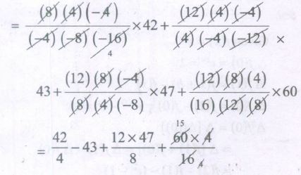
= \(\frac{21}{2}-43+70.5+15\)
= 10.5 - 43 + 70.5 + 15
y= 53
Hence when x = 15, f(x) = 53.
24.
Here total supply = 25 + 35 + 40 = 100
total requirement = 30 + 25 + 45 100
total supply = total requirement
∴ The given problem is a balanced transportation problem.
Hence, there exists a feasible solution for the given transportation problem.
North West Corner Rule:
I - allocation:
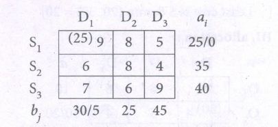
[∵ min (25, 30) = 25]
II - allocation:
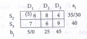
[∵ min (5, 35) = 5]
III - allocation:
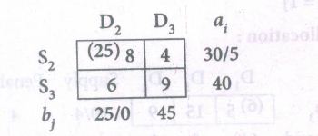
[∵ min (25, 30) = 25]
IV - allocation:
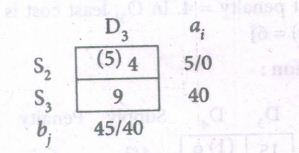
[∵ min (5, 45) = 5]
V - allocation:
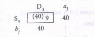
[∵ min (40, 40) = 40]
Thus, the allocations are
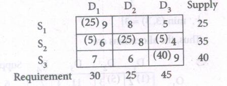
∴ The transportation schedule is
S1 → D1, S2 → D1, S2 → D2, S2 → D3, S3 → D3
Hence, the total transportation cost
= 25(9) + 5(6) + 25(8) + 5(4) + 40(9)
= 225 + 30 + 200 + 20 + 360
= Rs. 835
25.
Here the number of rows and columns are equal
∴ The given assignment problem is balanced.
Step 1 : Select a minimum element in each row and subtract this from all the elements in its row.
∴ The cost matrix of the given assignment problem is
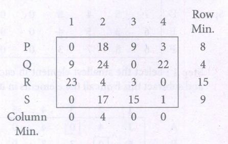
Column 2 has no zero. Go to Step 2.
Step 2 : Select the minimum element in each column and subtract this from all the elements in its column.
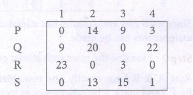
Since each row and column contains atleast one zero, assignments can be made.
Step 3 : Examine the rows with exactly one zero, mark it by and draw a vertical line.
After examining the rows, examine the columns with exactly one zero.
Mark it by and draw a horizontal line.
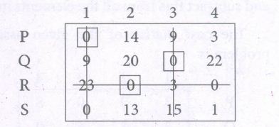
Only 3 assignments have been made.
The numbers not lying on the line are and min. is 1. Subtract 1 from all these numbers and add 1 to 23 which lies on the intersecting lines. Other numbers remain the same.
A new cost matrix is formed and repeat step 3.
∴ The new cost matrix is
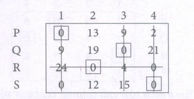
Thus, all the 4 assignments have been made.
∴The optimal assignment schedule and total cost is
| Subordinates | tasks | cost |
|---|---|---|
| P | 1 | 8 |
| Q | 3 | 4 |
| R | 2 | 19 |
| S | 4 | 10 |
| Total Cost | Rs. 41 | |
26.
\(\frac { dy }{ dx } \)+y cosx = 2 cosx
This is of the form \(\frac { dy }{ dx } \)+Py = Q where
P = cos x and Q = 2 cos x
\(\int { P } dx=\int { cosx } dx\) = sinx
Integrating factor (I.F.) = \(e^{ \int { P } dm }=e^{ sinx }\)
∴ The Solution is
\(ye^{ \int { P } dm }=\int { Q } e^{ \int { P } dm }dx\)
⇒ y esinx =\(\int { (2cosx){ e }^{ sinx } } dx\)+C
⇒ y esinx = 2\(\int { cosx } e^{ sinx }dx\)+C
⇒ y esinx = 2I1+C ..(1)
I1=\(\int { cosx } e^{ sinx }dx\)
put sin x = t ⇒ cos dx = dt
∴ It =\(\int { { e }^{ t } } dt\) = et = esinx
∴ (1) becomes, y esinx = 2.esinx + C
27.
\(\overline {\overline{X}} = \frac {5.10+4.98+5.02+4.96+4.96+5.04+4.94+4.92+4.92+4.98}{10}\)
\(\overline {\overline{X}}\) = \(\frac {49.82}{10} = 4.982\)
\(\overline {\overline{R}} = \frac {0.3+.4+.2+.4+.1+.1+.8+.5+.3+.5}{10}\)
\(\overline {R}\) = \(\frac {3.6}{10}\) = 0.36
The control limits of mean chart are
UCL = \(\overline {\overline{X}} + A_{2} \overline{R}\)
= 4.982 + .577(.36)
= 4.982+ .208 = 5.19
CL = 4.982
LCL = \(\overline {\overline{X}} - A_{2} \overline{R}\)
= 4.982 - .208 = 4.774
The control limits of R-chart are
UCL = D4\(\overline {R}\) = 2.114 (.36) = 0.761
CL = \(\overline {R}\) = .36
LCL = D3\(\overline {R}\) = 0
Mean Chart
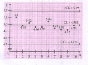
Range chart
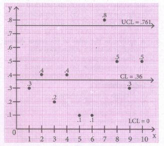
Conclusion: The above diagram shows all the control lines with the data points plotted.
Since one in Range chart, lie outside the control limits, we can say that the process is out of control.
28.
\(x\frac { dC }{ dx } =\frac { 3 }{ x } -C\)
\(x\frac { dC }{ dx } =\frac { 3 }{ x^2 } -\frac {C}{x}\)
\(\frac { dC }{ dx } +\frac { C }{ x } =\frac { 3 }{ { x }^{ 2 } } \)
i.e., \(\frac { dC }{ dx } +\frac { C }{ x } =\frac { 3 }{ { x }^{ 2 } } \)
It is of the form \(\frac { dC }{ dx } +PC=Q\)
Here, \(P=\frac { 1 }{ x } ,Q=\frac { 3 }{ { x }^{ 2 } } \)
ഽPdx = ഽ\(\frac 1 x\)dx = log x
I.F = eഽpdx = elog x = x
The Solution is
C(I.F) = ഽQ(I.F)dx + k where k is constant
Cx = ഽ\(\frac{3}{x^2}\)xdx + k
= 3ഽ\(\frac 1 x\) dx + k
Cx = 3log x + k (1)
Given C = 2 When x = 1
(1) ⇒ 2 × 1 ⇒ k =2
∴ The relationship between C and x is
Cx = 3 log x + 2
29.
| Commodities | Price | Quandity | p0q0 | p0q1 | p1q0 | p1q1 | ||
| 2003 (p0) |
2009 (q1) |
2003 (p0) |
2009 (q1) |
|||||
| Rice | 10 | 13 | 4 | 6 | 40 | 60 | 52 | 78 |
| Wheat | 125 | 18 | 7 | 8 | 105 | 120 | 126 | 144 |
| Rent | 25 | 29 | 5 | 9 | 125 | 225 | 145 | 261 |
| Fuel | 11 | 14 | 8 | 10 | 88 | 110 | 140 | 140 |
| Miscellaneous | 14 | 17 | 6 | 7 | 84 | 98 | 102 | 119 |
| Total | 442 | 613 | 537 | 742 | ||||
Fisher’s price index number
\({ P }_{ 01 }^{ F }=\left( \sqrt { \frac { \sum { { p }_{ 1 }{ q }_{ 10 } } \times \sum { { p }_{ 1 }{ q }_{ 1 } } }{ \sum { { p }_{ 0 }{ q }_{ 0 } } \times \sum { { p }_{ 0 }{ q }_{ 1 } } } } \right) \times 100=\left( \sqrt { \frac { 537\times 742 }{ 442\times 613 } } \right) \times 100=121.2684\)
Time Reversal Test:P01\(\times\) P10 = 1
\({ P }_{ 01 }\times { P }_{ 10 }=\sqrt { \left( \frac { \sum { { p }_{ 1 }{ q }_{ 0 } } \times \sum { { p }_{ 1 }{ q }_{ 1 } } \times \sum { { p }_{ 0 }{ q }_{ 1 } } \times \sum { { p }_{ 0 }{ q }_{ 0 } } }{ \sum { { p }_{ 0 }{ q }_{ 0 } } \times \sum { { p }_{ 0 }{ q }_{ 1 } } \times \sum { { p }_{ 1 }{ q }_{ 1 } } \times \sum { { p }_{ 1 }{ q }_{ 0 } } } \right) } \)
\({ P }_{ 01 }\times { P }_{ 10 }=\sqrt { \left( \frac { 537\times 742\times 613\times 442 }{ 442\times 613\times 742\times 537 } \right) } \)
\({ P }_{ 01 }\times { P }_{ 10 }=1\)
Factor Reversal Test
\({ P }_{ 01 }\times { Q }_{ 01 }=\frac { \sum { { p }_{ 1 }{ q }_{ 1 } } }{ \sum { { p }_{ 0 }{ q }_{ 0 } } } \)
\({ P }_{ 01 }\times { P }_{ 01 }=\sqrt { \left( \frac { \sum { { p }_{ 1 }{ q }_{ 0 } } \times \sum { { p }_{ 1 }{ q }_{ 1 } } \times \sum { { p }_{ 1 }{ q }_{ 0 } } \times \sum { { p }_{ 1 }{ q }_{ 1 } } }{ \sum { { p }_{ 0 }{ q }_{ 0 } } \times \sum { { p }_{ 0 }{ q }_{ 1 } } \times \sum { { p }_{ 0 }{ q }_{ 0 } } \times \sum { { p }_{ 0 }{ q }_{ 1 } } } \right) } \)
\({ P }_{ 01 }\times { P }_{ 01 }=\sqrt { \left( \frac { 537\times 742\times 613\times 742 }{ 442\times 613\times 442\times 537 } \right) } \)
\({ P }_{ 01 }\times { P }_{ 01 }=\sqrt { \left( \frac { 742\times 742 }{ 442\times 442 } \right) } =\frac { 742 }{ 442 } \Rightarrow { P }_{ 01 }\times { P }_{ 01 }=\frac { \sum { { p }_{ 1 }{ q }_{ 1 } } }{ \sum { { p }_{ 0 }{ q }_{ 0 } } } \)
30.
Sample size n = 100
Sample mean \(\bar { X } \)= 72
Population mean μ = 76
Population standard deviation σ = 8
Null Hypotheses H0:
μ = 76(i.e., There is no Significant difference between the state scores and the national scores)
\(Z=\frac { \bar { X } -\mu }{ \frac { \sigma }{ \sqrt { n } } } \)
\(\Rightarrow Z=\frac { 72-76 }{ \frac { 8 }{ \sqrt { 100 } } } =\frac { -4 }{ \frac { 8 }{ 10 } } =\frac { -4 }{ 8 } =-5\)
\(\Rightarrow |Z|=5\)
\({ Z }_{ \frac { \alpha }{ 2 } }=1.96\)
\(Z>{ Z }_{ \frac { \alpha }{ 2 } }i.e.,\ 5>1.96\)
Inference : Since \(Z>{ Z }_{ \frac { \alpha }{ 2 } }\) at 5% level of significance, the null hypothesis H0 is rejected.
Hence, we conclude that there is significant difference between the state scores and the national scores.
31.
Given Sample size n = 400
Sample mean \(\\ \bar { X } =67.47\)inches
Population mean μ = 67.39 & σ = 1.30 inches)
Null Hypotheses Ho:
μ = 67.39 inches (i.e., the sample has been drawn from the population with μ = 67.39 & σ = 1.30 inches)
Alternative Hypotheses H1:
μ ≠ 67.39 inches (two tail test)
(i.e., the sample has not been drawn from the population with μ = 67.39 & σ = 1.30 inches) The level of significance a = 5% = 0.05
Applying the test statistic,
\(Z=\frac { \bar { X } -\mu }{ \frac { \sigma }{ \sqrt { n } } } \)
\(\Rightarrow Z=\frac { 67.47-67.39 }{ \frac { 1.30 }{ \sqrt { 400 } } } =\frac { 0.08 }{ 0.065 } =1.2308\)
\(\therefore |Z|=1.2308\)
The significant value \({ Z }_{ \frac { \alpha }{ 2 } }=1.96\)
Here \(Z={ Z }_{ \frac { \alpha }{ 2 } }i.e.,1.2308<1.96\)
Inference: Since \({ Z }_{ \frac { \alpha }{ 2 } }\)at 5% level of significance the null hypothesis Ho is accepted.
Hence, we conclude that the sample has been drawn from the population with mean height 67.39 inches and standard deviation 1.30 inches.
32.
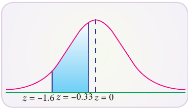
Given that mean μ = 150 and standard deviation σ = 15
(i) when X = 125 thousand
\(Z=\frac { X-\mu }{ \sigma } =\frac { 125-150 }{ 15 } =-1.667\)
When X = 145 thousand
\(Z=\frac { X-\mu }{ \sigma } =\frac { 145-150 }{ 15 } =-0.33\)
Area between Z = 0 and Z = -1.67 is 0.4525
Area between Z = 0 and Z = -0.33 is 0.1293
P(–1.667 ≤ Z ≤ –0.33) = 0.4525 – 0.1293
= 0.3232
Therefore the number of branches having sales between 125 thousand and 145 thousand is 550 × 0.3232 = 178
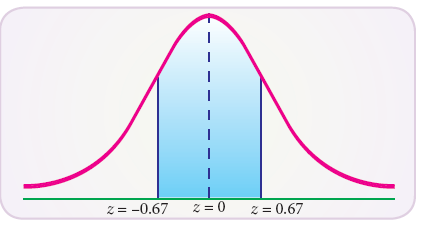
(ii) When X = 140 thousand
\(Z=\frac { X-\mu }{ \sigma } =\frac { 140-150 }{ 15 } =-0.67\)
When X = 160 thousand
\(Z=\frac { X-\mu }{ \sigma } =\frac { 160-150 }{ 15 } =0.67\)
P(–0.67 < Z < 0.67) = P(–0.67 < Z < 0) + P(0 < Z < 0.67)
= P(0 < Z < 0.67) + P(0 < Z < 0.67)
= 2 P(0 < Z < < 0.67)
= 2 × 0.2486
= 0.4972
Therefore, the number of branches having sales between Rs. 140 thousand and Rs. 160 thousand = 550 × 0.4972 = 273
33.
P = 1/5/100 = 1/500 = 0.002 n = 10 λ = np = 0.02
\(p(x)=\frac { { e }^{ -\lambda }{ \lambda }^{ x } }{ x! } =\frac { { e }^{ -0.02 }{ (0.02) }^{ x } }{ x! } \)
(i) Number of packets containing no defective = N p(o) = 1,00,000 × e–0.02
= 98020
(ii) Number of packets containing one defective = N p(1) = 1,00,000 × 0.9802 × 0.02
= 1960
(iii) Number of packets containing 2 defectives = N p(2) = 20
34.
Given p.d.f is = \(f(x)=\left\{\begin{array}{l} a+b x^{2}, 0 \leq x \leq 1 \\ 0, \text { otherwise } \end{array}\right.\)
Since f(x) is a p.d.f.\(\\ \int _{ -\infty }^{ \infty }{ f(x)dx=1 } \)
\(\Rightarrow \int _{ 0 }^{ 1 }{ (a+{ bx }^{ 2 })dx=1 } \)
\(\Rightarrow { \left[ ax+\frac { { bx }^{ 3 } }{ 3 } \right] }_{ 0 }^{ 1 }=1\Rightarrow a+\frac { b }{ 3 } =1\)
3a+b = 3 [multiplied by 3] ...(1)
Also it is given that E(X) = \(\frac{3}{5}\)
\(\Rightarrow \int _{ 0 }^{ 1 }{ x.f(x)dx=\frac { 3 }{ 5 } } \)
\(\Rightarrow \int _{ 0 }^{ 1 }{ (a+{ bx }^{ 2 })dx=\frac { 3 }{ 5 } } \)
\(\Rightarrow \int _{ 0 }^{ 1 }{ (ax+{ bx }^{ 3 })dx=\frac { 3 }{ 5 } } \)
\(\Rightarrow { \left[ \frac { { ax }^{ 2 } }{ 2 } +\frac { { bx }^{ 4 } }{ 4 } \right] }_{ 0 }^{ 1 }=\frac { 3 }{ 5 } \Rightarrow \frac { a }{ 2 } +\frac { b }{ 4 } =\frac { 3 }{ 5 } \)
\(\Rightarrow 2a+b=\frac { 12 }{ 5 } \) [Multiplies by 4] ...(2)
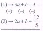
\(a=3-\frac { 12 }{ 5 } =\frac { 15-12 }{ 5 } =\frac { 3 }{ 5 } \)
Substituting a=\(\frac{3}{5}\) in(2) we get,
\(2(\frac { 3 }{ 5 } )+b=\frac { 12 }{ 5 } \Rightarrow \frac { 6 }{ 5 } +b=\frac { 12 }{ 5 } \)
\(\Rightarrow b=\frac { 12 }{ 5 } -\frac { 6 }{ 5 } =\frac { 6 }{ 5 } \)
\(\therefore a=\frac { 3 }{ 5 } ,b=\frac { 6 }{ 5 } \)
ii) \(E({ X }^{ 2 })=\int _{ 0 }^{ 1 }{ { x }^{ 2 }f(x)dx=\int _{ 0 }^{ 1 }{ { x }^{ 2 }\left( \frac { 3 }{ 5 } +\frac { 6 }{ 5 } { x }^{ 2 } \right) dx } } \)
\(\left[ \because a=\frac { 3 }{ 5 } ,b=\frac { 6 }{ 5 } \right] \)
\(=\int _{ 0 }^{ 1 }{ \left( \frac { 3 }{ 5 } { x }^{ 2 }+\frac { 6 }{ 5 } { x }^{ 4 } \right) dx } \)
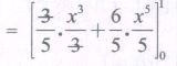
\(=\frac { 1 }{ 5 } (1-0)+\frac { 6 }{ 25 } (1-0)\)
\(=\frac { 1 }{ 5 } +\frac { 6 }{ 25 } =\frac { 5+6 }{ 25 } =\frac { 11 }{ 25 } \)
\(\therefore\) Var (X) = E(X2)-[E(X)]2
\(=\frac { 11 }{ 25 } -{ \left( \frac { 3 }{ 5 } \right) }^{ 2 }\)
\(=\frac { 11 }{ 25 } -\frac { 9 }{ 25 } =\frac { 2 }{ 25 } \)
\(\therefore\) Var (X) =\(\frac{2}{25}\)
35.
Let I = ∫ ex(1+x) log(xex)dx
Put t = x ex
⇒ dt = (x.ex + ex(1))dx
= ex(x+1)dx
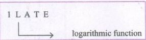
∴ I = ∫ log t.dt
Let u = log t; dv = dt
\(du=\frac { 1 }{ t } dt;v=t\)
∴Using integration by parts we get,
I = ∫udv = vu - ∫vdu
= t log t - ∫dt = t logt - t + c
= t log t - t + c
= xex log(xex) - (xex) + c [∵ t = xex]
= xex (log(xex)-1)+c
36.
\(\eta _{ d }=\frac { p+2{ p }^{ 2 } }{ 100-p-{ p }^{ 2 } } \)
\(\frac { -p }{ x } \frac { dx }{ dp } =\frac { p(2p+1) }{ 100-p-{ p }^{ 2 } } \)
\(\frac { -dx }{ x } =\frac { -(2p+1) }{ { p }^{ 2 }+p-100 } dp\)
\(\int { \frac { dx }{ x } } =\int { \frac { 2p+1 }{ { p }^{ 2 }+p-100 } } dp\)
log x = log(p2 + p = 100) + log k
ஃ x = k(p2 + p −100)
When x = 70, p = 5,
70 = k(25 + 5 − 100)
⇒ k = –1
Hence x = 100 − p − p2
R = px
Revenue = p(100 – p – p2)
37.
(a) We know that
\(\int _{ -\infty }^{ \infty }{ f(x) } dx=1\)
\(\int _{ 0 }^{ 10 }{ Axdx } +\int _{ 10 }^{ 20 }{ A(20-x)dx=1 } \)
\(A\left\{ { \left[ \frac { { x }^{ 2 } }{ 2 } \right] }_{ 0 }^{ 10 }+{ \left[ 20x-\frac { { x }^{ 2 } }{ 2 } \right] }_{ 10 }^{ 20 } \right\} =1\)
A[(50-0)+(400-200)-(200-50)] = 1
\(A=\frac{1}{100}\)
(b) (i) The probability that the number of pounds of bread that will be sold tomorrow is more than 10 pounds is given by
\(P(10\le X\le 20)=\int _{ 10 }^{ 20 }{ \frac { 1 }{ 100 } (20-x) } dx\)
\(=\frac { 1 }{ 100 } { \left[ 20x-\frac { { x }^{ 2 } }{ 2 } \right] }_{ 10 }^{ 20 }\)
\(=\frac { 1 }{ 100 } [(400-200)-(200-50)]\)
= 0.5
(ii) The probability that the number of pounds of bread that will be sold tomorrow is less than 10 pounds, is given by
\(P(0\le X\le 20)=\int _{ 0 }^{ 10 }{ \frac { 1 }{ 100 } } xdx\)
\(=\frac { 1 }{ 100 } { \left[ \frac { { x }^{ 2 } }{ 2 } \right] }_{ 0 }^{ 10 }\)
\(=\frac { 1 }{ 100 } (50-0)\)
= 0.5
(ii) The probability that the number of pounds of bread that will be sold tomorrow is between 5 and 15 pounds is
\(P(5\le X \le15)=\int _{ 5 }^{ 10 }{ \frac { 1 }{ 100 } xdx } +\int _{ 10 }^{ 15 }{ \frac { 1 }{ 100 } (20-x)dx } \)
\(=\frac { 1 }{ 100 } { \left[ \frac { { x }^{ 2 } }{ 2 } \right] }_{ 5 }^{ 10 }+\frac { 1 }{ 100 } { \left[ 20x-\frac { { x }^{ 2 } }{ 2 } \right] }_{ 10 }^{ 15 }\)
= 0.75
38.
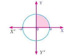
Equation of the required circle is \({ x }^{ 2 }+{ y }^{ 2 }={ a }^{ 2 }\) (1)
put \(y=0\), \({ x }^{ 2 }={ a }^{ 2 }\)
⇒ \(x=\pm a\)
Since equation (1) is symmetrical about both the axes
The required area = 4 [Area in the first quadrant between the limit 0 and a.]
\(=4\int _{ 0 }^{ a }{ y } \ dx\)
\(=4\int _{ 0 }^{ a }\sqrt { { a }^{ 2 }-{ x }^{ 2 } } dx=4{ \left[ \frac { x }{ 2 } \sqrt { { a }^{ 2 }-{ x }^{ 2 } } +\frac { { a }^{ 2 } }{ 2 } \sin ^{ -1 }{ \frac { x }{ a } } \right] }_{ 0 }^{ a }\)
\(=4{ \left[ 0+\frac { { a }^{ 2 } }{ 2 } \sin ^{ -1 }{( \frac { a }{ a } )} \right] }=4{ \left[ \frac { { a }^{ 2 } }{ 2 } \sin ^{ -1 }{( 1)} \right] }=4.\frac { { a }^{ 2 } }{ 2 }\frac { {π} }{ 2 }\)
= πa2 sq. units
39.
\(\int { { \left( \log x \right) }^{ 2 } } dx= \int { udv } \)
= uv − \(\int { } \)vdu
= x (log x)2 − 2\(\int { } \) logxdx...(*)
\(=x(\log x)^{ 2 }-2\int { udv } \)
\(=x(\log x)^{ 2 }-2[uv-\int { udv } ]\)
\(=x(\log x)^{ 2 }-2[x \log x-\int { dx] } \)
\(=x(\log x)^{ 2 }-2x \log x+x+c\)
\(=x[(\log{ ) }^{ 2 }-\log{ x }^{ 2 }+2]+c\)
| For \(\int { } \)log x dx in (*) | |
| Take u = (log x) Differentiate \(du=\frac { 1 }{ x } dx\) | and dv = dx Integrate v = x |
40.
(i) Transition probability matrix T = \(_{ E }^{ M }\left( \begin{matrix} \overset { M }{ 0.8 } & \overset { E }{ 0.2 } \\ 0.7 & 0.3 \end{matrix} \right) \)
After one study period, \(\left( \overset { M }{ 60\quad } \overset { E }{ 40 } \right) \) \(_{ E }^{ M }\left( \begin{matrix} \overset { M }{ 0.8 } & \overset { E }{ 0.2 } \\ 0.7 & 0.3 \end{matrix} \right) \) =\(\left( \overset { M }{ 76\quad } \overset { E }{ 24 } \right) \)
So in the very next study period, there will be 76 students do maths work and 24 students do the English work.
After two study periods,
\(\left( \overset { M }{ 76\quad } \overset { E }{ 24 } \right) \) \(_{ E }^{ M }\left( \begin{matrix} \overset { M }{ 0.8 } & \overset { E }{ 0.2 } \\ 0.7 & 0.3 \end{matrix} \right) \)
= (60.8+16.8 15.2+7.2)
= (77.6 22.4)
After two study periods there will be 78 (approx) students do maths work and 22 (approx) students do English work.

12th Standard Syllabus & Materials
12th Standard
TN 12th Computer Applications களப்பெயர் முறைமை (DNS) Sample Question Papers Study Material - QB365 Set A
NEW12th Standard
TN 12th Computer Applications வலையமைப்பு எடுத்துக்காட்டுகள் மற்றும் நெறிமுறைகள் Sample Question Papers Study Material - QB365 Set A
NEW12th Standard
TN 12th Computer Applications கணினி வலையமைப்பு ஓர் அறிமுகம் Sample Question Papers Study Material - QB365 Set A
NEW12th Standard
TN 12th Computer Applications PHP-உடன் MySQL-ஐ இணைத்தல் Sample Question Papers Study Material - QB365 Set A



Tamilnadu Stateboard 12th Standard Subjects

Maths

Chemistry

Physics

Biology

Computer Science
Business Maths and Statistics

Economics

Commerce

Accountancy

History

Computer Applications
Biology
Computer Technology
Computer Applications
Computer Science
Business Maths and Statistics
Commerce
Economics
Maths
Chemistry
Physics
Computer Technology
History
Accountancy

Tamil

English

French
Tamilnadu Stateboard Standards
