
 100% FREE ACCESS
12th Standard Syllabus & Materials
12th Standard
TN 12th Computer Applications மின்னணு தரவு பரிமாற்றம் Sample Question Papers Study Material - QB365 Set A
NEW12th Standard
TN 12th Computer Applications மின் - வணிக பாதுகாப்பு அமைப்புகள் Sample Question Papers Study Material - QB365 Set A
NEW12th Standard
TN 12th Computer Applications மின்னணு செலுத்தல் முறைகள் Sample Question Papers Study Material - QB365 Set A
NEW12th Standard
TN 12th Computer Applications மின் - வணிகம் Sample Question Papers Study Material - QB365 Set A
NEW12th Standard
TN 12th Computer Applications திறந்த மூல கருத்துருக்கள் Sample Question Papers Study Material - QB365 Set A
NEW12th Standard
TN 12th Computer Applications வலையமைப்பு வடமிடல் Sample Question Papers Study Material - QB365 Set A

Published on: 09/03/2020
12th Standard Business Mathamatics English Medium All Chapter Book Back and Creative Three Marks Questions 2020
Download Tamil Nadu 12th Standard Business Maths and Statistics question papers, model tests, one-mark questions, important questions, and public exam papers in PDF format. Free study materials and answer keys for TN State Board students.
Questions + Answers key
Take MCQ Business Maths and Statistics Test
1.
Calculate the seasonal indices for the following data by the method of simple average.
| Year | Quarters | |||
| I | II | III | IV | |
| 1994 | 78 | 66 | 84 | 80 |
| 1995 | 76 | 74 | 82 | 78 |
| 1996 | 72 | 68 | 80 | 70 |
| 1997 | 74 | 70 | 84 | 74 |
| 1998 | 76 | 74 | 86 | 82 |
2.
Fit a straight line trend for the following data using the method of least squares.
| x | 0 | 1 | 2 | 3 | 4 |
| y | 1 | 1 | 3 | 4 | 6 |
3.
The mean life time of 50 electric bulbs produced by a manufacturing company is estimated to be 825 hours with the S.D. of 110 hours. If II is the mean life time of all the bulbs produced by the company, test the hypothesis that μ = 900 hours at 5% level of significance.
4.
A random sample of marks in mathematics secured by 50 students out of 200 students showed a mean of 75 and a standard deviation of 10. Find the 95% confidence limits for the estimate of their mean marks.
5.
The life of army shoes is normally distributed with mean 8 months and standard deviation 2 months. If 5000 pairs are issued, how many pairs would be expected to need replacement within 12 months.
6.
Find the value of K if X is a normal variate whose p.d.f is given by f(x) = \(\frac { 1 }{ K } \)e8x-4x2, -∞
7.
Let X denote the number of hours you study during a randomly selected school day. The probability distribution function is
\(P(X=x)=\begin{cases} \begin{matrix} 0.1 & if\quad x=0 \end{matrix} \\ \begin{matrix} kx & if\quad x=1\quad or\quad 2 \end{matrix} \\ \begin{matrix} k(5-x) & if\quad x=3\quad or\quad 4 \end{matrix} \\ \begin{matrix} 0, & otherwise \end{matrix} \end{cases}\)
Find the value of k and what is the probability that you study atleast 2 hours.
8.
If a random variable. X has the probability distribution
| X | 0 | 1 | 2 | 3 | 4 | 5 |
| P(X=x) | a | 2a | 3a | 4a | 5a | 6a |
then find F(4)
9.
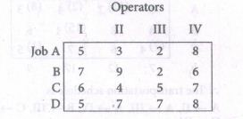
Solve the following assignment problem. Cell values represent cost of assigning job A, B, C and D to the operators I, II, III and IV.
10.
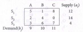
Find the initial basic feasible solution for the following transportation problem by Vogel's approximation method.
11.
Evaluate \(\int { \frac { { ({ a }^{ x }{ +b }^{ x }) }^{ 2 } }{ { a }^{ x }b^{ x } } dx } \)
12.
Evaluate \(\int { \frac { cos2x-cos2\alpha }{ cosx-cos\alpha } } dx\)
13.
Solve: (D2+1)y = 0 when x = 0, y = 2 and when x = \(\frac { \pi }{ 2 } \), y = -2.
14.
Solve: (x2-yx2)dy + (y2+xy2)dx = 0
15.
Find the number of men getting wages between Rs. 30 and Rs. 35 from the following table.
| Wages (x) | 20 - 30 | 30 - 40 | 40 - 50 | 50 - 60 |
| No. of men (y) | 9 | 30 | 35 | 42 |
16.
Using graphic method, find the value of y when x=27.
| x | 10 | 15 | 20 | 25 | 30 |
| y | 35 | 32 | 29 | 26 | 23 |
17.
The marginal revenue function is given by \(R'(x)=\frac { 3 }{ { x }^{ 2 } } -\frac { 2 }{ x } \). Find the revenue function and demand function if R(1) = 6
18.
Determine the cost of producing 3000 units of commodity if the marginal cost in rupees per unit is C'(x) = \(\frac{x}{3000}+2.50\)
19.
Solve: 2x + 3y = 5, 6x + 5y = 11
20.
If \(\left[ \begin{matrix} 1 & 0 & 0 \\ 0 & 0 & 1 \\ 0 & 1 & 0 \end{matrix} \right] \left[ \begin{matrix} x \\ y \\ z \end{matrix} \right] =\left[ \begin{matrix} 2 \\ -1 \\ 3 \end{matrix} \right] \) find x,y and z
21.
Find the rank of each of the following matrices.
\(\left( \begin{matrix} 3 & 1 & -5 \\ 1 & -2 & 1 \\ 1 & 5 & -7 \end{matrix}\begin{matrix} -1 \\ -5 \\ 2 \end{matrix} \right) \)
22.
Using graphic method, find the value of y when x = 48 from the following data:
| x | 40 | 50 | 60 | 70 |
| y | 6.2 | 7.2 | 9.1 | 12 |
23.
A farmer wants to decide which of the three crops he should plant on his 100-acre farm. The profit from each is dependent on the rainfall during the growing season. The farmer has categorized the amount of rainfall as high medium and low. His estimated profit for each is shown in the table.
| Rainfall | Estimated Conditional Profit(Rs.) | ||
| crop A | crop B | crop C | |
| High | 8000 | 3500 | 5000 |
| Medium | 4500 | 4500 | 5000 |
| Low | 2000 | 5000 | 4000 |
If the farmer wishes to plant only crop, decide which should be his best crop using
(i) Maximin
(ii) Minimax
24.
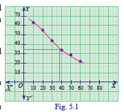
Using graphic method, find the value of y when x = 38 from the following data:
| x | 10 | 20 | 30 | 40 | 50 | 60 |
| y | 63 | 55 | 44 | 34 | 29 | 22 |
25.
Solve : (D2−4D−1)y = e−3x
26.
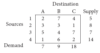
Obtain the initial solution for the following problem
27.
Explain the method of fitting a straight line.
28.
Write a brief note on seasonal variations
29.
A sample of 100 items, draw from a universe with mean value 4 and S.D 3, has a mean value 63.5. Is the difference in the mean significant at 0.05 level of significance?
30.
The standard deviation of a sample of size 50 is 6.3. Determine the standard error whose population standard deviation is 6?
31.
Integrate the following with respect to x
\(\frac { { e }^{ x } }{ { e }^{ 2x }-9 } \)
32.
If the chance of running a bus service according to schedule is 0.8, calculate the probability on a day schedule with 10 services :
(i) exactly one is late
(ii) atleast one is late
33.
34.
35.
The number of miles an automobile tire lasts before it reaches a critical point in tread wear can be represented by a p.d.f.
\(f(x)= \begin{cases}\frac{1}{30} e^{-\frac{x}{30}}, & \text { for } x>0 \\ 0, & \text { for } x \leq 0\end{cases}\)
Find the expected number of miles (in thousands) a tire would last until it reaches the critical tread wear point.
36.
Calculate consumer’s surplus if the demand function p = 122 − 5x − 2x2 and x = 6
37.
The marginal cost function of manufacturing x shoes is 6 +10x − 6x2. The cost producing a pair of shoes is Rs. 12. Find the total and average cost function.
38.
Evaluate \(\int { { e }^{ x }\left( { x }^{ 2 }+2x \right) dx } \)
39.
Find the rank of the matrix A = \(\left( \begin{matrix} 1 & 1 & 1 \\ 3 & 4 & 5 \\ 2 & 3 & 4 \end{matrix}\begin{matrix} 1 \\ 2 \\ 0 \end{matrix} \right) \)
40.
Find the order and degree of the following differential equations.
\(\frac{d^{3} y}{d x^{3}}+3\left(\frac{d y}{d x}\right)^{3}+2 \frac{d y}{d x}=0\)
1.
| Year | Quarters | |||
| I | II | III | IV | |
| 1994 | 78 | 66 | 84 | 80 |
| 1995 | 76 | 74 | 82 | 78 |
| 1996 | 72 | 68 | 80 | 70 |
| 1997 | 74 | 70 | 84 | 74 |
| 1998 | 76 | 74 | 86 | 82 |
| Total | 376 | 352 | 416 | 384 |
| Average | 75.2 | 70.4 | 83.2 | 76.8 |
Grand average = \(\frac {75.2+70.4+83.2+76.8}{4}\)
= \(\frac {305.6}{4}\) = 76.4
Seasonal index S.I = \(\frac {Quarterly average}{Grand average} \times 100\)
Hence, S.I for I quarter = \(\frac {75.2}{76.4} \times 100\) = 98.4
S.I for II quarter = \(\frac {70.4}{76.4} \times 100\) = 92.14
S.I for III quarter = \(\frac {83.2}{76.4} \times 100\) = 108.9
S.I for IV quarter = \(\frac {76.8}{76.4} \times 100\) = 100.5
2.
| x | y | x2 | xy |
| 0 | 1 | 0 | 0 |
| 1 | 1 | 1 | 1 |
| 2 | 3 | 4 | 6 |
| 3 | 4 | 9 | 12 |
| 4 | 6 | 16 | 24 |
| 10 | 15 | 30 | 43 |
Let y= ax + b be the best line of fit.
The normal equations are
a\(\sum\)x + nb = \(\sum\)y
a\(\sum\)x2 + b\(\sum\)x = \(\sum\)xy
10a+ 5b = 15
⇒ 2a+b = 3 ...(1)
30a + 10b = 43
⇒ 3a+b = 4.3 ....(2)
(1)-(2) ⇒ - a = -1.3
⇒ a = 1.3
Substituting a = 1.3 in (1) we get,
2(1.3) + b = 3
⇒ 2.6 + b = 3
⇒ b = 3 - 2.6 = 0.4
∴ The line of best fit isy = 1.3x + 0.4
3.
Given sample size n = 50
Sample mean \(\bar { x }\) = 825
Population mean μ = 900
Population S.D. σ = 110
Null hypotheses: H0: μ = 900
Alternative hypotheses: H1: μ ≠ 900
The test statistic, z = \(\frac { \bar { x } -\mu }{ \frac { \sigma }{ \sqrt { n } } } \)
=\(\frac { 825-900 }{ \frac { 110 }{ \sqrt { 50 } } } \) = -4.82
∴ |z| = -4.82
As the significance level is α = 0.05, \(Z_{ \frac { \alpha }{ 2 } }\) = 1.96
Here |z| > \(Z_{ \frac { \alpha }{ 2 } }\) as 4.82 > 1.96
Inference: As |z| > \(Z_{ \frac { \alpha }{ 2 } }\), H0 is rejected. Hence, we can conclude that mean life time of the population of electric bulbs cannot be taken as 900 hours.
4.
Sample size n = 50
Sample mean \(\bar { x } \) = 75
Sample S.D. s = 10
Standard error (S.E) = \(\frac { s }{ \sqrt { n } } =\frac { 10 }{ \sqrt { 50 } } =\frac { 10 }{ 7.07 } \)
= 1.414
As the significance level is α = 0.005, \(Z_{ \frac { \alpha }{ 2 } }\) = 1.96
∴ 95% confidence limits for the population mean is \(\bar { X } -Z_{ \frac { \alpha }{ 2 } }(S.E)\le \bar { X } -Z_{ \frac { \alpha }{ 2 } }(S.E)\)
⇒ 75 - (1.96)(1.414) ≤ μ ≤ 75 + (1.96)(1.414)
⇒ 75-2.771 ≤ μ ≤ 75 + 2.771
⇒ 72.23 ≤ μ ≤ 77.77
Hence, the 95% confidence interval of the population mean is (72.23, 77.77)
5.
Let X denote the life of army shoes.
Given μ = 8, σ = 2 and N = 5000
When μ = 12, Z = \(\frac { X-\mu }{ \sigma } =\frac { 12-8 }{ 2 } \) = 2
∴ P(X≤12) = P(Z≤2)
= P(-∞
P(X≤12) = 0.9772
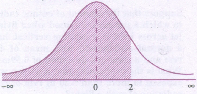
∴ The probability for a shoe need to be replaces is 0.9772.
∴ Out of 5000 pairs of shoes, number of pairs need to be replaced = 5000 \(\times\) 0.9772
= 4886.
6.
The p.d.f for the normal distribution is
f(x) = \(\frac { 1 }{ \sigma \sqrt { 2\pi } } .e^{ -\frac { 1 }{ 2 } \left( \frac { x-\mu }{ \sigma } \right) ^{ 2 } }\), -∞
f(x) = \(\frac { 1 }{ K } { e }^{ 8x-4x^{ 2 } }\)
= \(\frac { 1 }{ K } e^{ -4 }({ x }^{ 2 }-2x)\)
= \(\frac { 1 }{ K } e^{ -4 }({ x }^{ 2 }-2x+1-1)\)
\(\frac { 1 }{ K } e^{ -4 }(x-1)^{ 2 }+4\)
=\(\frac { 1 }{ K } .{ e }^{ 4 }e^{ -\frac { 1 }{ 2 } \frac { x-1^{ 2 } }{ \frac { 1 }{ 8 } } }\)
=\(\frac { 1 }{ 4 } { e }^{ 4 }e^{ -\frac { 1 }{ 2 } \left( \frac { x-1 }{ \frac { 1 }{ \sqrt { 8 } } } \right) ^{ 2 } }\) ...(2)
From (1) & (2), μ = 1, σ = \(\frac { 1 }{ \sqrt { 8 } } \) and
\(\frac { 1 }{ \sigma \sqrt { 2\pi } } =\frac { 1 }{ K } e^{ 4 }\)
\(\frac { 1 }{ \frac { 1 }{ \sqrt { 8 } } .\sqrt { 2 } \pi } =\frac { 1 }{ K } e^{ 4 }\)
⇒ \(\frac { \sqrt { 8 } }{ \sqrt { 2\pi } } =\frac { 1 }{ K } e^{ 4 }\)
\(\sqrt { \frac { 4 }{ \pi } } =\frac { 1 }{ K } { e }^{ 4 }\)
∴ K = \({ e }^{ 4 }\times \sqrt { \frac { \pi }{ 4 } } \)
7.
The probability distribution of X is
| X | 0 | 1 | 2 | 3 | 4 |
| P(X) | 0.1 | k | 2k | 2k | k |
Σpi = 1 ⇒ 0.1 + k + 2k + 2k + k = 1
⇒ 0.1 + 6k = 1 ⇒ 6k = 1-0.1 = 0.9
⇒ k = \(\frac{0.9}{6}\) = 0.15
And the probability that you study atleast 2 hours is P(X≥2)=P(X=2)+P(X=3)+P(X=4)
= 2k + 2k + k = 5k
= 5(0.15) = 0.75
8.
Since the random variable X is the probability distribution function, Σpi = 1
∴ a + 2a + 3a + 4a + 5a + 6a = 1
21a = 1 ⇒ a = \(\frac{1}{21}\)
Now, F(4) = P(X ≤ 4)
= P(X = 0) + P(X = 1) + P(X = 2)P(X = 3) + P(X = 4)
= a + 2a + 3a + 4a + 5a = 15a
= 15\((\frac{1}{21})=\frac{5}{7}\)
∴ F(4) = \(\frac{5}{7}\)
9.
Here the number of rows and columns are equal.
∴ The given assignment problem is balanced.
Step 1 :
Select a minimum element in each row and subtract this from all the elements in its row.
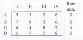
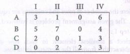
Here IV column has no zero. Go to step 2.
Step 2:
Select the minimum element in each column and subtract this from all the elements in its column.
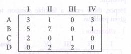
Since each row and column contains atleast one zero, assignments can be made.
Step 3:
Examine the rows with only one zero. Mark that. zero by and draw a vertical line.
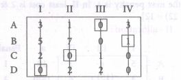
Thus, all the assignments have been made.
The optimal assignment schedule and total cost is
| Job | Operator | Cost |
|---|---|---|
| A | III | 2 |
| B | IV | 6 |
| C | II | 4 |
| D | I | 5 |
| Total Cost | Rs. 17 | |
10.
Σai = 12 + 14 + 4 = 30
Σbj = 9 + 10 + 11 = 30
Σai = Σbj
∴ The given problem is a balanced transportation problem.
Hence, there exists a feasible solution to the given problem.
I - allocation :
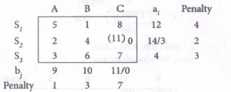
[∵ the highest penalty is 7, In C, least cost is 0 & min (11, 14) = 11]
II - allocation :
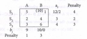
[∵ the highest penalty is 4, In S1'least cost is 1& min (10, 12) = 10]
III - allocation :
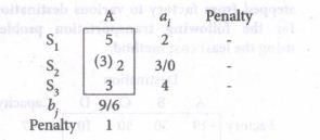
[∵ In A, least cost is 2 & min (9, 3) = 3]
IV - allocation :
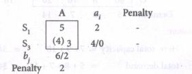
[∵ In A, least cost is 3 & min (6,4) = 4]
V - allocation :
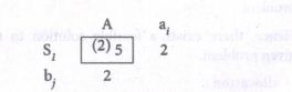
[∵ min (2, 2) = 2]
Thus, the allocations are
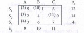
∴ The transportation schedule is
S1 → A, S1 → B, S2 → A, S2 → C S3 → A
Hence, the total transportation cost is
= 2(5) + 10(1) + 3(2) + 11(0) + 4(3)
= 10 + 10 + 6 + 0 + 12 = Rs. 38
11.
\(\int { \frac { { ({ a }^{ x }{ +b }^{ x }) }^{ 2 } }{ { a }^{ x }b^{ x } } dx } \) = \(\int { \frac { { a }^{ 2x }+{ b }^{ 2x }+{ 2a }^{ x }{ b }^{ x } }{ { 2a }^{ x }{ b }^{ x } } } \)
[∵ (a + b)2 = a2 + 2ab + b2]
= \(\int { \left( \frac { { a }^{ 2 }x }{ { a }^{ x }{ b }^{ x } } +\frac { { b }^{ 2x } }{ { a }^{ x }{ b }^{ x } } +\frac { 2{ a }^{ x }{ b }^{ x } }{ { a }^{ x }{ b }^{ x } } \right) } dx\)
= \(\int { \left( \frac { { a }^{ x } }{ { b }^{ x } } +\frac { { b }^{ x } }{ { a }^{ x } } +2 \right) dx } \)
= \(\int { \left( { \left( \frac { a }{ b } \right) }^{ x }+{ \left( \frac { b }{ a } \right) }^{ x }+2 \right) } dx\)
= \(\frac { { \left( \frac { a }{ b } \right) }^{ x } }{ { log }_{ e }\left( \frac { a }{ b } \right) } +\frac { { \left( \frac { b }{ a } \right) }^{ 2 } }{ { log }_{ e }\left( \frac { b }{ a } \right) } +2x+c\)
12.
\(\int { \frac { cos2x-cos2\alpha }{ cosx-cos\alpha } } dx\)
= \(\frac { ({ 2cos }^{ 2 }x-1)-({ 2cos }^{ 2 }\alpha -1) }{ cos\quad x-cos\alpha } dx\)
= \(\frac { { 2cos }^{ 2 }x-cos^{ 2 }\alpha }{ cos\quad x-cos\alpha } \)
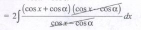
= \(2\int { (cos\quad x+cos\alpha )dx } \)
= \(2[sinx+cos\alpha .x]+c\)
= \(2sinx+2xcos\alpha +c\)
13.
The auxiliary equation is m2 + 1 = 0
⇒ m2 = -1
⇒ m = ±\(\sqrt { -1 } \) = ±i
Here α = 0, β = 1
∴ CF is e0x [A cosx + B sinx]
∴ The general solution is
y = A cos x + B sin x ...(1)
Given when x = 0, y = 2
∴ 2 = A cos 0 + B sin 0
⇒ 2 = A+0 ⇒ A = 2
[∵ cos0 = 1 and sin0 = 0]
Also, when x = \(\frac { \pi }{ 2 } \), y = -2
∴ -2 = A\(cos\frac { \pi }{ 2 } +Bsin\frac { \pi }{ 2 } \)
⇒ -2 = A(0)(+B(1) ⇒ B = -2
[∵ \(cos\frac { \pi }{ 2 } \) = 0 and \(sin\frac { \pi }{ 2 } \)= 1]
Substituting the values of A & B in (1) we get,
y = 2 cos x - 2 sin x
⇒ y = 2 (cosx - sin x)
14.
Given (x2-yx2)dy + (y2+xy2)dx = 0
⇒ x2(1-y)dy+y2(1+x)dx = 0
⇒ x2(1-y)dy = -y2(1+x)dx
Separating the variables we get,
\(\frac { (1-y) }{ y^{ 2 } } dy=-\frac { (1+x) }{ x^{ 2 } } \)dx
⇒ \(\frac { 1 }{ { y }^{ 2 } } dy-\frac { 1 }{ y } dy=-\frac { 1 }{ x^{ 2 } } dx-\frac { 1 }{ x } dx\)
Integrating, \(\int { { y }^{ -2 } } dy-\int { \frac { 1 }{ y } } dy=-\int { \frac { 1 }{ x^{ 2 } } } dx-\int { \frac { 1 }{ x } } \)
\(-\frac { 1 }{ y } -logy=\frac { 1 }{ x } \) -log x + C
⇒ log x - log y = \(\frac { 1 }{ x } +\frac { 1 }{ y } \)+C
⇒ log \(log\left( \frac { x }{ y } \right) =\frac { x+y }{ xy } \)+C
⇒ \(\frac { x }{ y } =e^{ \frac { x+y }{ xy } +C }\)
⇒ \(\frac { x }{ y } =K.e^{ \frac { x+y }{ xy } }\) [where eC = K]
15.
Let us calculate the number of men whose wages is less than Rs. 35 by using Newton's forward interpolation formula
xo + nh = x ⇒ 30 + n (10) = 35
⇒ 10n = 35 - 30 = 5
⇒ n = \(\frac{5}{10}\) = 0.5
The difference table is
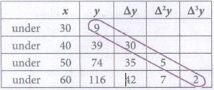
\(\Rightarrow { y }_{ o }+\frac { n }{ n! } \triangle { y }_{ o }+\frac { n(n+1) }{ 2! } { \triangle }^{ 2 }{ y }_{ o }+\frac { n(n+1)(n-2) }{ 3! } { \triangle }^{ 3 }{ (y }_{ o })\)
\(y(35)=9+\frac { 0.5 }{ 1! } (30)+\frac { (0.5)(0.5-1) }{ 2 } (5)+\frac { (0.5)(0.5-1)(0.5-2) }{ 6 } (2)\)
= 9 + 15 - 0.6 + 0.1 = 24 (approximately)
∴ Number of men getting wages between Rs. 30 and Rs. 35 is y(35) - y(30) = 24 - 9 = 15.
16.
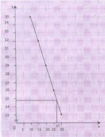
From the graph, it is clear that when x = 27, the value of y is 24.8
17.
Given \(R'(x)=\frac { 3 }{ { x }^{ 2 } } -\frac { 2 }{ x } \)
\(\Rightarrow \int { R'(x) } =\int { \left( \frac { 3 }{ { x }^{ 2 } } -\frac { 2 }{ x } \right) } dx\)
\(\Rightarrow R(x)=\frac { -3 }{ x } -2log\quad x+k\)
Given R(1) = 6 ⇒ when x = 1, R = 6
\(\Rightarrow 6=\frac { -3 }{ 1 } -2log1+k\)
⇒ 6 + 3 = k [∵ log 1 = 0]
⇒ k = 9
\(\therefore R(x)=-\frac { 3 }{ x } -2log\quad x+9\)
Demand function \(P=\frac { R }{ x } \)
\(\\ =\frac { 3 }{ { x }^{ 2 } } -\frac { 2log\quad x }{ x } +\frac { 9 }{ x } \)
18.
Given, marginal cost, C' (x) \(\frac{x}{3000}+2.50\)
\(\int { C'(x) } =\int { \left( \frac { x }{ 300 } +2.50 \right) dx } \)
\(C(x)=\frac { { x }^{ 2 } }{ 6000 } +2.50x+k\)
When x = 0, c = 0 ⇒ k = 0
∴ c(x) = \(\frac{x^2}{6000}+2.50x\)
When x = 3000
Cost of production
\(=\frac { { (3000) }^{ 2 } }{ 6000 } +2.50(3000)\)
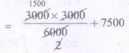
= 1500 + 7500
= Rs. 9000
19.
Given non-homogeneous equations are
2x + 3y = 5 6X + 5y = 11
\(\Delta =\left| \begin{matrix} 2 & 3 \\ 6 & 5 \end{matrix} \right| =10-18=-8\)
Since \(\Delta \neq 0\) Cramer's rule can be applied and the system is consistent with unique solution
\(\Delta x=\left| \begin{matrix} 5 & 3 \\ 11 & 5 \end{matrix} \right| =25-33=-8\)
\(\Delta y=\left| \begin{matrix} 2 & 5 \\ 6 & 11 \end{matrix} \right| =22-30=-8\)
\(\therefore x=\cfrac { \Delta x }{ \Delta } =\cfrac { -8 }{ -8 } =1\)
\(y=\cfrac { \Delta y }{ \Delta } =\cfrac { -8 }{ -8 } =1\)
\(\therefore \) Solution set is {1, 1}
20.
\(\left[ \begin{matrix} 1 & 0 & 0 \\ 0 & 0 & 1 \\ 0 & 1 & 0 \end{matrix} \right] \left[ \begin{matrix} x \\ y \\ z \end{matrix} \right] =\left[ \begin{matrix} 2 \\ -1 \\ 3 \end{matrix} \right] \)
\(\Rightarrow \left( \begin{matrix} x0+0 \\ 0+0+z \\ 0+y+0 \end{matrix} \right) =\left( \begin{matrix} 2 \\ -1 \\ 3 \end{matrix} \right) \)
\(\Rightarrow \left( \begin{matrix} x \\ y \\ z \end{matrix} \right) =\left( \begin{matrix} 2 \\ -1 \\ 3 \end{matrix} \right) \)
\(\Rightarrow x=2\quad z=-1\quad y=3\)
\(\therefore\) Solution set is {2,3, -1}
21.
A =\(\left( \begin{matrix} 3 & 1 & -5 \\ 1 & -2 & 1 \\ 1 & 5 & -7 \end{matrix}\begin{matrix} -1 \\ -5 \\ 2 \end{matrix} \right) \)
The order of A is 3 x 4
\(\therefore \rho (A)\le \text{minimum} \ of(3,4)\)
\(\therefore \rho (A)\le 3\)
Let us transform the matrix A to an echelon form
| Matrix A | Elementary Transformation |
|---|---|
| \(A=\left( \begin{matrix} 3 & 1 & -5 \\ 1 & -2 & 1 \\ 1 & 5 & -7 \end{matrix}\begin{matrix} -1 \\ -5 \\ 2 \end{matrix} \right) \) | |
| \(\sim \left( \begin{matrix} 1 & 5 & -7 \\ 1 & -2 & 1 \\ 3 & 1 & -5 \end{matrix}\begin{matrix} 2 \\ -5 \\ -1 \end{matrix} \right) \) | \({ R }_{ 1 }\leftrightarrow { R }_{ 3 }\) |
| \(\sim \left( \begin{matrix} 1 & 5 & -7 \\ 0 & -7 & 8 \\ 3 & 1 & -5 \end{matrix}\begin{matrix} 2 \\ -7 \\ -1 \end{matrix} \right) \) | \({ R }_{ 2 }\rightarrow { R }_{ 2 }+{ R }_{ 1 }\) |
| \(\sim \left( \begin{matrix} 1 & 5 & -7 \\ 0 & -7 & 8 \\ 0 & -14 & 16 \end{matrix}\begin{matrix} 2 \\ -7 \\ -7 \end{matrix} \right) \) | \({ R }_{ 3 }\rightarrow { R }_{ 3 }+{ 3R }_{ 1 }\) |
| \(\sim \left( \begin{matrix} 1 & 5 & -7 \\ 0 & -7 & 8 \\ 0 & 0 & 0 \end{matrix}\begin{matrix} 2 \\ -7 \\ 7 \end{matrix} \right) \) | \({ R }_{ 3 }\rightarrow { R }_{ 3 }-{ 2R }^{ 2 }\) |
The matrix is in echelon form and the number of non-zero matrix is 3
\(\therefore \rho (A)=3\)
22.
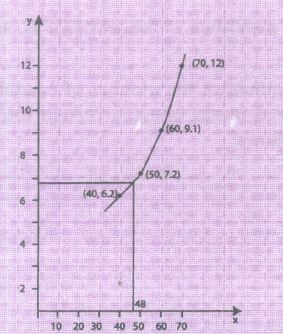
Scale:
In x axis 1 cm = 10 units
In y axis 1 cm = 2 units
Plot the points (40, 6.2), (50, 7.2), (60, 9.1) and (70, 12). At x = 48, draw a vertical line to the graph and from the intersecting point, draw a horizontal line to meet the y-axis
From the graph, we find that when x = 48, the value of Y is equal to 6.8.
23.
| Estimated Conditional Profit 0 | |||||
| Rainfall | High | Medium | Low | Minimum payoff | Maximum payoff |
| Crop A | 8000 | 4500 | 2000 | 2000 | 8000 |
| Crop B | 3500 | 4500 | 5000 | 3500 | 5000 |
| Crop C | 5000 | 5000 | 4000 | 4000 | 5000 |
(i) Max (2000,3500,4000) = 4000
∴ Crop C is the best according to maximin criteria
(ii) Min (8000,5000,5000) = 5000
∴ Crop B and C are best according to minimax criteria
24.
(i) Take a suitable scale for the values of x and y, and plot the various points on the graph paper for given values of x and y.
(ii) Draw a suitable curve passing through the plotted points.
(iii) Find the point corresponding to the value x = 38 on the curve and then read the corresponding value of y on the y- axis, which will be the required interpolated value.
From the graph in Figure we find that for x = 38, the value of y is equal to 35
25.
(D2−4D−1)y = e−3x
The auxiliary equation is
m2−4m−1 = 0
(m−2)2−4−1 = 0
(m− 2)2 = 5
\(m-2=±\sqrt { 5 } \)
\(m=2±\sqrt5\)
C.F = Ae\((2+\sqrt5)x\) + Be\((2-\sqrt5)x\)
\(PI=\frac { 1 }{ \phi (D) } f(x)\)
= \(\frac { 1 }{ { D }^{ 2 }-4D-1 } { e }^{ -3x }\)
\(=\frac { 1 }{ { (-3) }^{ 2 }-4(-3)-1 } { e }^{ -3x }\) (Replace D by −3)
\(=\frac { 1 }{ 9+12-1 } { e }^{ -3x }\)
\(=\frac { e^{ -3x } }{ 20 } \)
Hence the general solution is y = C.F+P.I
⇒ y = Ae\((2+\sqrt5)x\) + Be\((2-\sqrt5)x\)+\(\frac { e^{ -3x } }{ 20 } \)
26.
Here total supply = 5 + 8 + 7 + 14 = 34, Total demand = 7 + 9 + 18 = 34
(i.e) Total supply =Total demand
Therefore The given problem is balanced transportation problem.
\(\therefore\) we can findan initial basic feasible solution to the given problem.
From the above table we can choose the cell in the North West Corner. Here the cell is (1, A)
Allocate as much as possible in this cell so that either the capacity of first row is exhausted or the destination requirement of the first column is exhausted.
i.e. x11 = min (5, 7) = 5
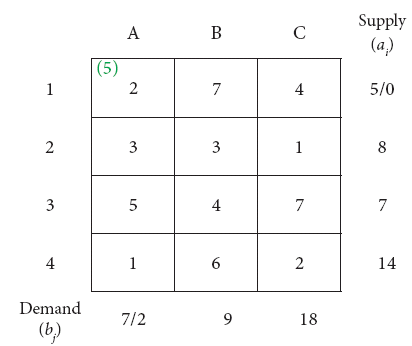
Reduced transportation table is
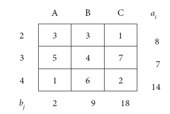
Now the cell in the North west corner is (2, A)
Allocate as much as possible in the first cell so that either the capacity of second row is exhausted or the destination requirement of the first column is exhausted.
i.e. x12 = min (2, 8) = 2
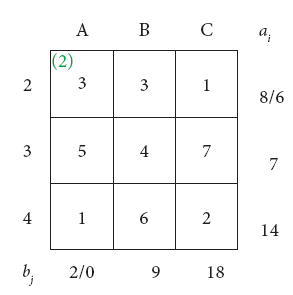
Reduced transportation table is
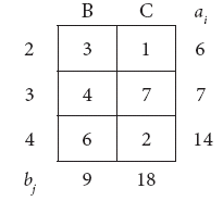
Here north west corner cell is (2, B) Allocate as much as possible in the first cell so that either the capacity of second row is exhausted or the destination requirement of the second column is exhausted.
i.e. x22 = min (6, 9) = 6
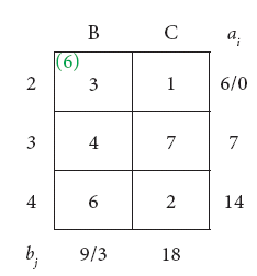
Reduced transportation table is
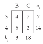
Here north west corner cell is (3,B).
Allocate as much as possible in the first cell so that either the capacity of third row is exhausted or the destination requirement of the second column is exhausted.
i.e. x32 = min (7, 3) = 3
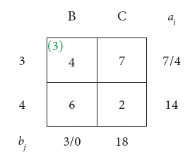
Reduced transportation table is
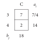
Here north west corner cell is (3,C) Allocate as much as possible in the first cell so that either the capacity of third row is exhausted or the destination requirement of the third column is exhausted.
i.e. x33 = min (4, 18) = 4
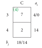
Reduced transportation table and final allocation is x44 = 14
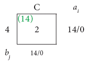
Thus we have the following allocations
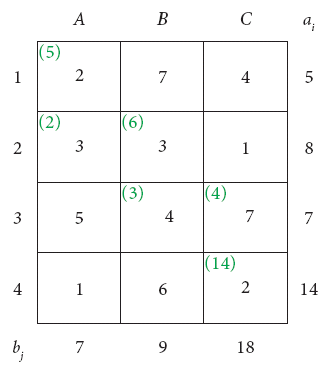
Transportation schedule : 1⟶A, 2⟶B, 3⟶B, 3⟶C, 4⟶C
The total transportation cost.
= (5 \(\times\) 2) + (2 x\(\times\) 3) + (6 \(\times\) 3) + (3 \(\times\) 4) + (4 \(\times\) 7) + (14 \(\times\) 2)
= Rs. 102
27.
The line of least fit is a line from which the sum of the deviations of various points is zero. This is the best method for obtaining the trend values.
(i) The straight line trend is represented by
Y = a + b X ...(1)
where Y is the actual value and X is time
(ii) The constants 'a' and 'b' are estimated by solving the following two normal Equations
\(\sum\) Y = n a + b \(\sum\) X
\(\sum\) XY = a\(\sum\) X + b \(\sum\) X2 where n is the number of years given in the data.
(iii) By substituting the values of 'a' and 'b' in the trend equation (1), we get the line of best fit.
28.
Tendency movements are due to nature, which repeat themselves periodically in every seasons. These variations repeat themselves in less than one year time. It is measured in an interval of time.
Seasonal variations may be influenced by natural force, social customs and traditions.
29.
Sample size n = 100,
Sample mean \(\\ \bar { X } =3.5\)
Population mean μ = 4
Population standard deviation σ = 3
Null Hypotheses: There is no significant difference in the mean. i.e., Ho : μ = 4
Alternative Hypotheses : There is Significant difference in the mean.
i.e., H1 : μ ≠ H
The level of significance ∝ = 5% = 0.05
Applying the test statistic,\(Z=\frac { \bar { X } -\mu }{ \frac { \sigma }{ \sqrt { n } } } \)
\(\Rightarrow Z=\frac { 3.5-4 }{ \frac { 3 }{ \sqrt { 100 } } } =\frac { -.5 }{ .3 } =-1.667\)
\(\Rightarrow |Z|=1.667\)
\({ Z }_{ \frac { \alpha }{ 2 } }=1.96\)
Here Z < \({ Z }_{ \frac { \alpha }{ 2 } }\)i.e., 1.667<1.96
Inference: Since Z<\({ Z }_{ \frac { \alpha }{ 2 } }\)at 5% level of significance, the null hypothesis H0 is accepted. Hence there is no Significant difference in the mean.
30.
Sample size n = 50
Sample S.D s = 6.3
Population S.D \(\sigma\) = 6
The standard error for sample S.D is given by
\(S.E=\sqrt { \frac { { \sigma }^{ 2 } }{ 2n } } =\frac { 6 }{ \sqrt { 2(50) } } =\frac { 6 }{ \sqrt { 100 } } =0.6\)
Thus standard error for sample S.D = 0.6.
31.
\(Let\ I=\int { \frac { { e }^{ x }dx }{ { e }^{ 2x }-9 } } dx\)
\(=\int { \frac { { e }^{ x }dx }{ { \left( { e }^{ x } \right) }^{ 2 }-9 } } \)
\(Put\ { e }^{ x }=t\Rightarrow { e }^{ x }dx=dt\)
\(\therefore I=\int { \frac { dt }{ { t }^{ 2 }-9 } } =\int { \frac { dt }{ { t }^{ 2 }-{ 3 }^{ 2 } } } \)
\(=\frac { 1 }{ 2\times 3 } \log { \left| \frac { t-3 }{ t+3 } \right| } +c\)
\(\left[ \because \int { \frac { dx }{ { x }^{ 2 }-{ a }^{ 2 } } } =\frac { 1 }{ 2a } \log { \left| \frac { x-a }{ x+a } \right| } +c \right] \)
\(=\frac { 1 }{ 6 } \log { \left| \frac { { e }^{ x }-3 }{ { e }^{ x }+3 } \right| } +c\)
32.
Probability of bus running late is denoted as p = 1-0.8 = 0.2
Probability of bus running according to the schedule is q = 0.8
Also given that n = 10
The binomial distribution is p(x) = 10Cx(0.2)x(0.8)10-x
(i) probability that exactly one is late P(x = 1) = 10C1pq9
= 10C1(0.2)(0.8)9
(ii) probability that at least one is late
= 1 – probability that none is late
= 1 – p(x = 0)
= 1– (0.8)10
33.
34.
35.
Given p.d.f is
\(f(x)= \begin{cases}\frac{1}{30} e^{-\frac{x}{30}}, & \text { for } x>0 \\ 0, & \text { for } x \leq 0\end{cases}\)
Expected number of miles
\(E(X)=\int _{ -\infty }^{ \infty }{ x.f(x)dx } \)
\(=\int _{ 0 }^{ \infty }{ x.\frac { 1 }{ 30 } { e }^{ \frac { -x }{ 30 } }dx=\int _{ }^{ \infty }{ { xe }^{ \frac { -x }{ 36 } }dx } } \)
\(\left[ \because \int _{ 0 }^{ \infty }{ { x }^{ n }{ e }^{ -axdx }=\frac { n! }{ { a }^{ n+1 } } Hence\quad n=1,a=\frac { 1 }{ 30 } } \right] \)
\(=\frac { 1 }{ 30 } \left( \frac { 1! }{ { \left( \frac { 1 }{ 30 } \right) }^{ 2 } } \right) \)
\(=\frac { 1 }{ 30 } \times \frac { 1 }{ { \left( \frac { 1 }{ 30 } \right) }^{ 2 } } =\frac { 1 }{ \frac { 1 }{ 30 } } =30\)
∴ E(X) = 30 miles (in thousands) or 30,000 miles.
36.
Given demand functionp = 122 - 5x - 2x2 and x = 6
When x0 = 6, p0 = 122-5(6)-2(6)2
= 122-30-72
= 122-102
P0 = 20
p0x0 = 20 \(\times\) 6 = 120
Consumer's Surplus
CS \(=\int _{ 0 }^{ x }{ f(x) } dx-{ p }_{ 0 }{ x }_{ 0 }\)
\(=\int _{ 0 }^{ 6 }{ (122-5x-2{ x }^{ 2 })dx-120 } \)
\(={ \left[ 122x-\frac { 5{ x }^{ 2 } }{ 2 } -\frac { { 2x }^{ 3 } }{ 3 } \right] }_{ 0 }^{ 6 }-120\)
\(=122(6)-5\frac { \left( { 6 }^{ 2 } \right) }{ 2 } -2\frac { \left( { 6 }^{ 3 } \right) }{ 3 } -120\)
\(=732-\frac { 180 }{ 2 } -\frac { 432 }{ 3 } -120\)
= 732-90-144-120
= 732-354
C.S = 378 units
37.
Given,
Marginal cost MC = 6 +10x − 6x2
C = \(\int { MC } dx+k\)
= \(\int { (6+10x-{ 6x }^{ 2 })dx+k } \)
= 6x + 5x2 − 2x3 + k (1)
when x = 2, C = 12 (given)
12 = 12 + 20 −16 + k
k = -4
C = 6x + 5x2 − 2x3 − 4
Average cost = \(\frac { C }{ x } =\frac { 6x+{ 5x }^{ 2 }-2{ x }^{ 3 }+{ 4 } }{ x } \)
= 6 + 5x − 2x2 − \(\frac { 4 }{ x } \)
38.
\(\int { { e }^{ x }\left( { x }^{ 2 }+2x \right) dx } =\int { { e }^{ x }\left[ f(x)+f'(x) \right] } dx\)
= ex f(x) + c
= ex x2 + c
[Take f(x) = x2
\(\therefore\) f'(x) = 2x]
39.
The order of A is 3 \(\times\) 4.
\(\therefore \) \(\rho (A)\le 3.\)
Let us transform the matrix A to an echelon form
| Matrix A | Elementary Transformation |
| \(A=\left( \begin{matrix} 1 & 1 & 1 \\ 3 & 4 & 5 \\ 2 & 3 & 4 \end{matrix}\begin{matrix} 1 \\ 2 \\ 0 \end{matrix} \right) \) \(\sim \left( \begin{matrix} 1 & 1 & 1 \\ 0 & 1 & 2 \\ 0 & 1 & 2 \end{matrix}\begin{matrix} 1 \\ -1 \\ -2 \end{matrix} \right) \) \(\sim \left( \begin{matrix} 1 & 1 & 1 \\ 0 & -1 & -2 \\ 0 & 0 & 0 \end{matrix}\begin{matrix} 1 \\ 1 \\ -1 \end{matrix} \right) \) |
\({ R }_{ 2 }\rightarrow { R }_{ 2 }-{ 3R }_{ 1 }\) \({ R }_{ 3 }\rightarrow { R }_{ 3 }-{ 2R }_{ 1 }\) \({ R }_{ 3 }\rightarrow { R }_{ 3 }-{ R }_{ 2 }\) |
The number of non zero rows is 3.
\(\therefore \) \(\rho (A)=3.\)
40.
The highest derivative is third order and its power is one
∴ order : 3,
degree : 1

12th Standard Syllabus & Materials
12th Standard
TN 12th Computer Applications களப்பெயர் முறைமை (DNS) Sample Question Papers Study Material - QB365 Set A
NEW12th Standard
TN 12th Computer Applications வலையமைப்பு எடுத்துக்காட்டுகள் மற்றும் நெறிமுறைகள் Sample Question Papers Study Material - QB365 Set A
NEW12th Standard
TN 12th Computer Applications கணினி வலையமைப்பு ஓர் அறிமுகம் Sample Question Papers Study Material - QB365 Set A
NEW12th Standard
TN 12th Computer Applications PHP-உடன் MySQL-ஐ இணைத்தல் Sample Question Papers Study Material - QB365 Set A



Tamilnadu Stateboard 12th Standard Subjects

Maths

Chemistry

Physics

Biology

Computer Science
Business Maths and Statistics

Economics

Commerce

Accountancy

History

Computer Applications
Biology
Computer Technology
Computer Applications
Computer Science
Business Maths and Statistics
Commerce
Economics
Maths
Chemistry
Physics
Computer Technology
History
Accountancy

Tamil

English

French
Tamilnadu Stateboard Standards
