
 100% FREE ACCESS
12th Standard Syllabus & Materials
12th Standard
TN 12th Computer Applications மின்னணு தரவு பரிமாற்றம் Sample Question Papers Study Material - QB365 Set A
NEW12th Standard
TN 12th Computer Applications மின் - வணிக பாதுகாப்பு அமைப்புகள் Sample Question Papers Study Material - QB365 Set A
NEW12th Standard
TN 12th Computer Applications மின்னணு செலுத்தல் முறைகள் Sample Question Papers Study Material - QB365 Set A
NEW12th Standard
TN 12th Computer Applications மின் - வணிகம் Sample Question Papers Study Material - QB365 Set A
NEW12th Standard
TN 12th Computer Applications திறந்த மூல கருத்துருக்கள் Sample Question Papers Study Material - QB365 Set A
NEW12th Standard
TN 12th Computer Applications வலையமைப்பு வடமிடல் Sample Question Papers Study Material - QB365 Set A

Published on: 03/09/2022
QB365 provides a detailed and simple solution for every Possible Book Back Questions in Class 12 Business Maths Subject - Applied Statistics, English Medium. It will help Students to get more practice questions, Students can Practice these question papers in addition to score best marks.
Download Tamil Nadu 12th Standard Business Maths and Statistics question papers, model tests, one-mark questions, important questions, and public exam papers in PDF format. Free study materials and answer keys for TN State Board students.
Questions + Answers key
Take MCQ Business Maths and Statistics Test
1.
Write the control limits for the R chart.
2.
Write the control limits for the mean chart.
3.
What are the uses of statistical quality control?
4.
Define R Chart.
5.
Define mean chart.
6.
Name the control charts for variables.
7.
Define a control chart.
8.
What do you mean by process control?
9.
What do you mean by product control?
10.
Define Assignable Cause.
11.
Define Chance Cause.
12.
Mention the types of causes for variation in a production process.
13.
Define Statistical Quality Control.
14.
State the uses of Cost of Living Index Number.
15.
Define Family Budget Method.
16.
Discuss about Cost of Living Index Number.
17.
Define true value ratio.
18.
Explain Factor Reversal Test.
19.
Define Time Reversal Test.
20.
State the test of adequacy of index number.
21.
Write note on Fisher’s price index number.
22.
Explain Paasche’s price index number.
23.
Define Laspeyre’s price index number.
24.
Mention the classification of Index Number.
25.
State the uses of Index Number.
26.
Define Index Number.
27.
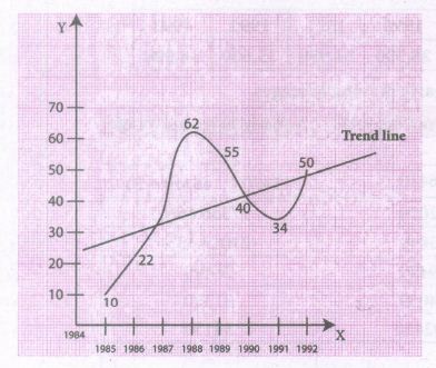
The following table gives the number of small-scale units registered with the Directorate of Industries between 1985 and 1991. Show the growth on a trend line by the free hand method.
| Years | 1985 | 1986 | 1987 | 1988 | 1989 | 1990 | 1991 | 1992 |
| No. of units (in‘000) | 10 | 22 | 36 | 62 | 55 | 40 | 34 | 50 |
28.
Find the trend of production by the method of a five-yearly period of moving average for the following data:
| Year | 1979 | 1980 | 1981 | 1982 | 1983 | 1984 | 1985 | 1986 | 1987 | 1988 | 1989 | 1990 |
| Production(‘000) | 126 | 123 | 117 | 128 | 125 | 124 | 130 | 114 | 122 | 129 | 118 | 123 |
29.
State the two normal equations used in fitting a straight line.
30.
Define seasonal index.
31.
Discuss about irregular variation
32.
Explain cyclic variations.
33.
Define secular trend.
34.
Mention the components of the time series.
35.
State the uses of time series.
36.
What is the need for studying time series?
37.
Define Time series.
38.
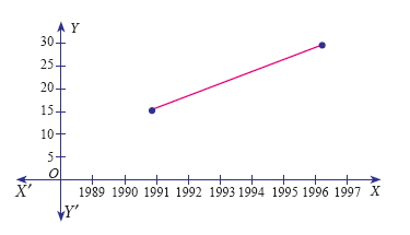
Fit a trend line by the method of semi-averages for the given data.
| Year | 1990 | 1991 | 1992 | 1993 | 1994 | 1995 | 1996 | 1997 |
| Sales | 15 | 11 | 20 | 10 | 15 | 25 | 35 | 30 |
39.
1.
| Case (i) when SD are given |
Case (ii) when SD are not given |
| (i) UCL = \(\overline{R} + 3 {\sigma}_{R}\) | (i) UCL = D4 \(\overline {R }\) |
| (ii) CL = \(\overline {R }\) | (ii) CL = \(\overline {R }\) |
| (iii) LCL = \(\overline {R} - {3\sigma_{R}}\) | (iii) LCL = D3 \(\overline {R }\) |
2.
The control limits for mean chart in two different cases are :
| Case (i) when \(\overline {X }\) and SD are given |
Case (ii) when \(\overline {X }\) and SD are not given |
| (i) UCL = \({\overline{X}} + 3 \frac{\sigma}{\sqrt n}\) | (i) UCL = \(\overline {X }\) + A2 \(\overline {R }\) |
| (ii) CL = \(\overline {X }\) | (ii) CL = \({\overline {X }}\) |
| (iii) LCL = \({\overline{X}} - \frac{3\sigma}{\sqrt n}\) | (iii) LCL = \(\overline {X }\) - A2 \(\overline {R }\) |
3.
I. It is a powerful technique used to diagnose the lack of quality in any of the raw materials, process, machines etc.
II. It is essential that the end products should possess the qualities that the consumer expects from the manufacturer.
4.
The R chart is to show the variability or dispersion of the samples taken from the given process.
5.
The mean chart is to show the quality averages of the samples taken from the given process
6.
The control charts of variables are
(i) Charts for mean (\(\overline { X } \))
(ii) Charts for Range (R)
7.
The statistical tool applied in process control is the Control Chart. Control Charts are the devices to describe the patterns of variation. It is an instrument to be used in specitication, production and inspection and is the core of statistical quality control. It is essentially a graphic device, simple to construct and easy to interpret.
8.
The main objective in any product process is to control and maintain a satisfactory quality level of the manufactured product. This is done by Process Control. In process control the proportion of defective items in the production process is to be minimized and it is achieved through the technique of control charts.
9.
Product control means that controlling the quality of the product by critical examination through sampling inspection plans. It aims at a certain quality level to be guaranteed to the customers. It attempts to ensure that the product sold does not contain a large number of defective items.
10.
Assignable Causes is present in any production process is due to non-random causes. It may occur at any stage of the process, right from the arrival of the raw materials to the final delivery of the product. Some of the important factors of assignable causes are defective raw materials, fault in machines. unskilled manpower, worn out tools, new operation etc.
11.
Chance Causes are small variations which are natural and inherent in the manufacturing process. The variation occurring due to these causes is beyond the human control and cannot be prevented or eliminated under any circumstances. The minor causes which do not affect the quality of the products to an extent are called as Chance Causes or Random Causes. For example Rain, floods, power cuts, etc
12.
There are two causes of variation which affects the quality of the product namely
(i) Chance causes (or) Random causes
(ii) Assignable causes.
13.
Statistical Quality control is a powerful technique used to diagnose the lack of quality in any of the raw materials, processes, machines etc. It is essential that end products should possess the qualities that the consumer expects from the manufacturer.
14.
(i) It indicates whether the real wages of workers are rising or falling for a given time.
(ii) It is used by the administrators for regulating dearness allowance or grant of bonus to the workers.
15.
In this method, the weights are calculated by multiplying prices and quantity of the base year.
Cost of living index number = \(\frac {\sum pV}{\sum V}\) where
P = \(\frac {p_{1}}{p_{0}} \times 100 \) is the price relative and
V = \(\sum p_{0}q_{0}\) is the value relative
16.
Cost of Living Index Number is constructed to study the effect of changes in the price of goods and services of consumers for a current period as compared with the base period. The change in the cost of living index number between any two periods means the change in income which will be necessary to maintain the same standard of living in both the periods. Therefore the cost of living index number measures the average increase in the cost to maintain the same standard of life.
Further, the consumption habits of people differ widely from class to class (rich, poor, middle class) and even with the region. The changes in the price level affect the different classes of people, consequently, the general price index numbers fail to reflect the effect of changes in their cost of living in different classes of people. Therefore, the cost of living index number measures the general price movement of the commodities consumed by different classes of people.
17.
The ratio between the total value of current period and total value of the base period is known as true value ratio.
(\( \frac{\sum P_{1} q_{1}}{\sum p_{0} q_{0}}\) is a true value tario)
18.
Factor reversal test is another test for testing the consistency of a good index number. The product of price index number and quantity index number from the base year to the current year should be equal to the true value ratio. That is ratio between the total value of current period and total value of the base period is known as true value ratio. Factor reversal test is given by,
\(\text { i.e. } P_{01} \times Q_{01}=\frac{\sum P_{1} q_{1}}{\sum p_{0} q_{0}}=V_{01}(\text { Except the factor 100) }\)
19.
Time reversal test is an important test for testing the consistency of a good index number. This test maintains time consistency by working both forward and backward with respect to time (here time refers to base year and current year). Symbolically the following Relationship should be satisfied, P01 \(\times\) P10 = 1 Fisher's index number formula satisfies the above relationship
\(\text { i.e. } P_{01}=\frac{1}{P_{10}} \text { or } P_{01} \times P_{10}=1(\text { Except the factor } 100 \text { ) }\)
20.
Index numbers are studied to know the relative changes in price and quantity for any two years compared. There are two tests which are used to test the adequacy for an index number. The two tests are as follows.
(i) Time reversal test
(ii) Factor reversal test
The criterion for a good index number is to satisfy the above two tests.
21.
Fisher's price index number is the geometric mean of Laspeyre's and Paasche's price index number. Hence it is weighted index number.
Fisher's price index number = \(\sqrt {\frac {\sum p_{1}q_{0}}{\sum p_{0}q_{0} }}{\times}{\frac {\sum p_{1}q_{1}}{\sum p_{0}q_{1}} \times {100}}\)
22.
In Paasche's price index number, the quantity of the current year is used as weight.
Paasche's price index number
\(P^{p}_{01}\) = \(\frac {\sum p_{1}q_{1}}{\sum p_{0}q_{1}} \times {100}\)
23.
The weighted aggregate index number using base period weights is called Laspeyre’s price index number.
\(P_{01}^{L}=\frac{\sum p_{1} q_{0}}{\sum p_{0} q_{0}} \times 100\)
Where p1 is current year price
p0 is base year price
q0 is base year quantity
24.
Index number can be classified as follows
(i) Price index number
It measures the general changes in the retail or wholesale price level of a particular or group of commodities.
(ii) Quantity index number
These are indices to measure the changes in the quantity of goods manufactured in a factory.
(iii) Cost of living index number
These are intended to study the effect of change in the price level on the cost of living of diferent classes of people.
25.
(i) It is an important tool for the formulating decision and management policies
(ii) It helps in studying the trends and tendencies
(iii) It determines the inflation and deflation in an economy
26.
An index numberis a device which shows by its variations the changes in a magnitude which is not capable of accurate measurements in itself or of direct valuation in practice
27.
28.
| Year | Production ('000) | 5 yearly Total column | 5 yearly moving average |
|---|---|---|---|
| 1979 | 126 | - | - |
| 1980 | 123 | - | |
| 1981 | 117 | 619 | 123.8 |
| 1982 | 128 | 617 | 123.4 |
| 1983 | 125 | 624 | 124.8 |
| 1984 | 124 | 621 | 124.2 |
| 1985 | 130 | 615 | 123 |
| 1986 | 114 | 619 | 123.8 |
| 1987 | 122 | 613 | 122.6 |
| 1988 | 129 | 606 | 121.2 |
| 1989 | 118 | - | - |
| 1990 | 123 | - | - |
29.
The two normal equations are
\(\sum\) Y = n a + b \(\sum\) X
\(\sum\) XY = a \(\sum\) X + b \(\sum\)X2 where n is the number of years given in the data.
30.
Seasonal index is a measure of how a particular season compares with the average season.
31.
Irregular variations do not have particular pattern and there is no regular period of time of their occurrences. Normally they are short terms variations but its occurrence sometimes has its effect so intense that they may give rise to new cyclic or other movements of variations.
For example floods, wars, earthquakes, Tsunami, strikes, lockouts etc.
32.
Cyclic uniformly periodic in nature. They may or may not follow exactly similar patterns after equal intervals of time. Generally one cyclic period ranges from 7 to.9 years and there is no hard and fast rule in the fixation of years for a cyclic period. For example, every business cycle has a Start-Boom-Depression- Recover maintenance during booms and depressions, changes in government monetary policies, changes in interestrates.
33.
It is a general tendency of time series to increase or decrease or stagnates during a long period of time. An upward tendency is usually observed in population of a country, production, sales, prices in industries, income of individuals etc., A downward tendency is observed in deaths,epidemics, prices of electronic gadgets, water sources, mortality rate etc. It is not necessarily that the increase or decrease should be in the same direction throughout the given period of time. This feature is known as secular trend.
34.
The components of time series are
(i) Secular trend
(ii) Seasonal variations
(iii) Cyclic variations
(iv) Irregular variations
35.
Time series has an important objective to identify the variations and try to eliminate the variations and also helps us to estimate or predict the future values.
36.
(i) It helps in the analysis of the past behavior
(i) It helps in forecasting and for future plans
(ii) It helps in the evaluation of current achievements
(iv) It helps in making comparative studies between one time period and others
37.
A time series consists of a set of observations arranged in chronological order (either ascending or descending). It is a statistical data which relates to successive intervals or point of time.
38.
Since the number of years is even(eight), we can equally divide the given data it two equal parts and obtain the averages of first four years and last four years.
| Year | Production | Average |
| 1990 | 15 | \(\frac{15+11+20+10}{4}=14\) |
| 1991 | 11 | |
| 1992 | 20 | |
| 1993 | 10 | |
| 1994 | 15 | \(\frac{15+25+35+30}{4}=26.25\) |
| 1995 | 25 | |
| 1996 | 35 | |
| 1997 | 30 |
39.

12th Standard Syllabus & Materials
12th Standard
TN 12th Computer Applications களப்பெயர் முறைமை (DNS) Sample Question Papers Study Material - QB365 Set A
NEW12th Standard
TN 12th Computer Applications வலையமைப்பு எடுத்துக்காட்டுகள் மற்றும் நெறிமுறைகள் Sample Question Papers Study Material - QB365 Set A
NEW12th Standard
TN 12th Computer Applications கணினி வலையமைப்பு ஓர் அறிமுகம் Sample Question Papers Study Material - QB365 Set A
NEW12th Standard
TN 12th Computer Applications PHP-உடன் MySQL-ஐ இணைத்தல் Sample Question Papers Study Material - QB365 Set A



Tamilnadu Stateboard 12th Standard Subjects

Maths

Chemistry

Physics

Biology

Computer Science
Business Maths and Statistics

Economics

Commerce

Accountancy

History

Computer Applications
Biology
Computer Technology
Computer Applications
Computer Science
Business Maths and Statistics
Commerce
Economics
Maths
Chemistry
Physics
Computer Technology
History
Accountancy

Tamil

English

French
Tamilnadu Stateboard Standards
