
 100% FREE ACCESS
12th Standard Syllabus & Materials
12th Standard
TN 12th Computer Applications மின்னணு தரவு பரிமாற்றம் Sample Question Papers Study Material - QB365 Set A
NEW12th Standard
TN 12th Computer Applications மின் - வணிக பாதுகாப்பு அமைப்புகள் Sample Question Papers Study Material - QB365 Set A
NEW12th Standard
TN 12th Computer Applications மின்னணு செலுத்தல் முறைகள் Sample Question Papers Study Material - QB365 Set A
NEW12th Standard
TN 12th Computer Applications மின் - வணிகம் Sample Question Papers Study Material - QB365 Set A
NEW12th Standard
TN 12th Computer Applications திறந்த மூல கருத்துருக்கள் Sample Question Papers Study Material - QB365 Set A
NEW12th Standard
TN 12th Computer Applications வலையமைப்பு வடமிடல் Sample Question Papers Study Material - QB365 Set A

Published on: 03/09/2022
QB365 provides a detailed and simple solution for every Possible Creative Questions in Class 12 Business Maths Subject - Applied Statistics, English Medium. It will help Students to get more practice questions, Students can Practice these question papers in addition to score best marks.
Download Tamil Nadu 12th Standard Business Maths and Statistics question papers, model tests, one-mark questions, important questions, and public exam papers in PDF format. Free study materials and answer keys for TN State Board students.
Questions + Answers key
Take MCQ Business Maths and Statistics Test
1.
In a line of best fit, find the slope and y intercept if \(\Sigma X=10, \Sigma Y=25, \Sigma X^{2}=35, \Sigma X Y=90\) and n = 5.
2.
Fit the line of best fit if \(\Sigma X=75, \Sigma Y=115\), \(\Sigma \mathrm{X}^{-2}=1375, \Sigma X Y=1875\) and n = 6.
3.
In a straight line of best fit find x-intercept when \(\Sigma X=10, \Sigma Y=16.9, \Sigma X^{2}=30, \Sigma X Y=47.4\) n = 7
4.
Fit a straight line to the following \(\Sigma \mathrm{I}=10, \Sigma Y=19, \Sigma \mathrm{X}^{2}=30, \Sigma \mathrm{XY}=53\) and n = 5
5.
Calculate the seasonal index by the method of simple average for the following data.
| Year | I Quarter | II Quarter | III Quarter | Iv Quarter |
| 1985 | 65 | 60 | 61 | 63 |
| 1986 | 68 | 55 | 66 | 61 |
| 1987 | 68 | 60 | 63 | 67 |
6.
Below are given figures of production (in thousand tonnes) of a sugar factory. Obtain the trend values by 3 year moving average.
| Year | 1980 | 1981 | 1982 | 1983 | 1984 | 1985 | 1986 |
| Production | 80 | 90 | 92 | 83 | 94 | 99 | 92 |
7.
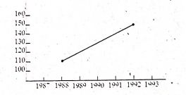
Fit a trend line by method of semi averages.
| Year | 1987 | 1988 | 1989 | 1990 | 1991 | 1992 | 1993 |
| Production (in tonnes) |
90 | 110 | 130 | 150 | 100 | 150 | 200 |
8.
From the data given below calculate seasonal indices.
| Year | I Quarter | II Quarter | III Quarter | Iv Quarter |
| 1985 | 68 | 62 | 61 | 63 |
| 1986 | 65 | 58 | 66 | 61 |
| 1987 | 68 | 63 | 63 | 67 |
9.
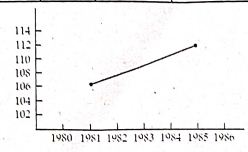
Fit a trend line by the method of semi averages
| Year | 1980 | 1981 | 1982 | 1983 | 1984 | 1985 | 1986 |
| Sales | 102 | 105 | 114 | 110 | 108 | 116 | 112 |
10.
The following data shows the value of sample mean (\(\bar{X}\)) and the range R for 10 samples of size 5 each. Calculate the control limits for : mean chart and range chart.
| Sample No. | 1 | 2 | 3 | 4 | 5 | 6 | 7 | 8 | 9 | 10 |
| Mean \(\bar{X}\) | 11.2 | 11.8 | 10.8 | 11.6 | 11.0 | 9.6 | 10.4 | 9.6 | 10.6 | 10.0 |
| Range | 7 | 4 | 8 | 5 | 7 | 4 | 8 | 4 | 7 | 9 |
(Given for n = 5, A2 = .577, D3 = 0, D4 = 2.115)
11.
Construct the cost of living index for 2003 on the basis of 2000 from the following data using family budget method.
| Item | Price(Rs.) | Weights | |
| Food | 2000 | 2003 | 30 |
| Rent | 200 | 280 | 30 |
| Clothing | 150 | 120 | 20 |
| Fuel & lighting | 50 | 100 | 10 |
| Miscellaneous | 100 | 200 | 20 |
12.
Calculate the cost of living index by aggregate expenditure method
| Commodity | Quantity | Price(Rs.) | |
| 2000 | 2000 | 2003 | |
| A | 100 | 8 | 12 |
| B | 25 | 6 | 7.50 |
| C | 10 | 5 | 5.25 |
| D | 20 | 48 | 52 |
| E | 65 | 15 | 16.50 |
| F | 30 | 19 | 27.00 |
13.
Calculate the seasonal indices by the method of simple average for the following data.
| Year | I quarter | II quarter | III quarter | IV quarter |
| 1985 | 68 | 62 | 61 | 63 |
| 1986 | 65 | 58 | 66 | 61 |
| 1987 | 68 | 63 | 63 | 67 |
14.
Calculate the 3-yearlymoving averages of the production figures (in tonnes) for the following data.
| Year | 1973 | 1974 | 1975 | 1976 | 1977 | 1978 | 1979 | 1980 | 1981 | 1982 | 1983 | 1984 | 1985 | 1986 | 1987 |
| Production | 15 | 21 | 30 | 36 | 42 | 46 | 50 | 56 | 63 | 70 | 74 | 82 | 90 | 95 | 102 |
15.
Using the method ofleast squares, fit a straight line trend for Σx = 10, Σy = 16.9, Σx2 = 30, Σxy = 47.4 and n = 7.
1.
The line of best fit is Y = aX + b
The normal equation are
\(
a \Sigma X^{2}+b \Sigma X =\Sigma X Y
\)
\(a \Sigma X+n b =\Sigma Y
\)
30a + 10b = 90 ..... (1)
10a+ 5b = 25 ...... (2)
Solving (1) and (2) we get
a = 4, b = -3
The line of best fit Y = 4X - 3 and y intercept = -3.
2.
The line of best fet is Y = aX+b
\(
\Sigma Y a= \Sigma X+n b
\)
\(\Sigma X Y =a \Sigma X^{2}+b \Sigma X\)
115 75a + 6b ..............(1)
1875 1375a + 75b ................(2)
Solving (1) and (2)
a = 1, b = 6.6667
Y = X + 6.6667
3.
The line of best fit is Y = aX+ b
The normal equations are
\(
\Sigma Y =a \Sigma X+n b
\)
\(\Sigma X Y =a \Sigma X^{2}+b \Sigma X\)
10a +7b = 16.9 .......... (1)
30a + 10b = 47.4 .........(2)
Solving (1) and (2) we get,
a = 1.48, b = 0.3
The line of best fit is Y = 1.482x + 0.3.
The x intercept of the line of best fit is \(-\frac{0.3}{1.48}\)
4.
The line of best fit is Y = aX + b
The normal equations are
\(
\sum Y =a \sum X+n b
\)
\(\sum X Y =a \sum X^{2}+b \sum X
\)
10a + 5b = 19 ............(1)
30a + 10b = 53 ..............(2)
Solving (1) and (2) we get
a = 1.5 and b = 0.8
The line of best fit is Y = 1.5X + 0.8.
5.
| Year | Quarter | |||
| I | II | III | IV | |
| 1985 | 65 | 60 | 61 | 63 |
| 1986 | 68 | 55 | 66 | 61 |
| 1987 | 68 | 60 | 63 | 67 |
| Total | 201 | 175 | 190 | 191 |
| Average | 67 | 58.333 | 63.33 | 63.67 |
Grand average \(
=\frac{252.33}{4}=63.08
\)
Seasonal Index (S.I) \( =\frac{\text { Quarterly Average }}{\text { Grand Average }} \times 100
\)
S.I for I Quarter \(
=\frac{67}{63.08} \times 100
=106.21 \%
\)
S.I for II Quarter \( =\frac{58.33}{63.08} \times 100
=92.7 \%
\)
S.I for III Quarter \( =\frac{63.33}{63.08} \times 100
=100.4 \%
\)
S.I for IV Quarter \( =\frac{63.67}{63.08} \times 100
=100.94 \%
\)
6.
| Year | Production | 3 yearly moving total | 3 yearly moving average |
| 1980 | 80 | - | - |
| 1981 | 90 | 262 | 87.33 |
| 1982 | 92 | 265 | 88.33 |
| 1983 | 83 | 269 | 89.67 |
| 1984 | 94 | 276 | 92 |
| 1985 | 99 | 285 | 95 |
| 1986 | 92 | - | - |
7.
| Year | Production | Semi Total | Semi Average |
| 1987 | 90 | ||
| 1988 | 110 | 330 | 110 |
| 1989 | 130 | ||
| 1990 | 150 | ||
| 1991 | 100 | ||
| 1992 | 150 | 450 | 150 |
| 1993 | 200 |
8.
| Year | Quarter | |||
| I | II | III | IV | |
| 1985 | 68 | 62 | 61 | 63 |
| 1986 | 65 | 58 | 66 | 61 |
| 1987 | 68 | 63 | 63 | 67 |
| Total | 201 | 183 | 190 | 191 |
| Average | 67 | 61 | 63.333 | 63.67 |
Grand average = \(\frac{255}{4}=63.75\)
Seasonal Index (S.I) \( =\frac{\text { Quarterly Average }}{\text { Grand Average }} \times 100
\)
S.I for I Quarter \( =\frac{67}{63.75} \times 100=105.01
\)
S.I for II Quarter \( =\frac{61}{63.75} \times 100=95.68 \)
S.I for III Quarter \( =\frac{6.3 .333}{6.3 .75} \times 100=99.35
\)
S.I for IV Quarter = \(\frac{63.67}{63.75} \times 100=99.87 \)
9.
| Year | Sales | Semi Total | Semi average |
| 1980 | 102 | ||
| 1981 | 105 | 321 | 107 |
| 1982 | 114 | ||
| 1983 | 110 | ||
| 1984 | 108 | ||
| 1985 | 116 | 336 | 112 |
| 1986 | 112 |
10.
\(\bar{\bar{X}}\) = \(\frac{11.2 + 11.8 + 10.8 + 11.6 + 11.0+ 9.6 + 10.4 + 9.6 + 10.6 + 10.0}{10}\)
\(=\frac{106.6}{10}=10.66\)
\(\bar{R}=\frac{7+4+8+5+7+4+8+4+7+9}{10}\)
\(=\frac{63}{10}=6.3\)
Control limits for mean chart
UCL = \(\bar{\bar{X}}\) + A2\(\bar{R}\)
= 10.66 + .577(6.3) = 14.295
CL = \(\bar{\bar{X}}\) = 10.66
Control limits for R-chart
UCL = D2\(\bar{R}\) = 2.115 \(\times\) 6.3
= 13.324
CL = \(\bar{R}\) = 6.3
LCL = D3\(\bar{R}\) = 0
11.
| Items | p0 | p1 | Weights V | \(P=\frac{p_1}{p_0}\times100\) | PV |
| Food | 200 | 280 | 30 | 140 | 4200 |
| Rent | 100 | 200 | 20 | 200 | 4000 |
| Clothing | 150 | 120 | 20 | 80 | 1600 |
| Fuel & Lighting | 50 | 100 | 10 | 200 | 2000 |
| Miscellaneous | 100 | 200 | 20 | 200 | 4000 |
| 100 | 15800 |
Cost of living index (C.L.I) = \(\frac{\Sigma PV}{\Sigma V}\)
= \(\frac{15800}{100}\) = 158
Hence, there is 58% increase in cost of living in 2003 compared to 2000.
12.
| Commodity | Quantity | Price(Rs.) | p1q0 | p0q0 | |
| 2000(q0) | 2000 (p0) | 2003 (p1) | |||
| A | 100 | 8 | 12 | 1200 | 800 |
| B | 25 | 6 | 7.50 | 187.50 | 150 |
| C | 10 | 5 | 5.25 | 52.50 | 50 |
| D | 20 | 48 | 52 | 1040.00 | 960 |
| E | 65 | 15 | 16.50 | 1072.50 | 975 |
| F | 30 | 19 | 27.00 | 810 | 570 |
C.L.I = \(\frac{\Sigma p_1q_0}{\Sigma p_0q_0}\times100\)
C.L.I = \(\frac{4362.50}{3505}\times100\) = 124.46
13.
| Year | I quarter | II quarter | III quarter | IV quarter |
| 1985 | 68 | 62 | 61 | 63 |
| 1986 | 65 | 58 | 66 | 61 |
| 1987 | 68 | 63 | 63 | 67 |
| Total | 201 | 183 | 190 | 191 |
| Average | 67 | 61 | 63.33 | 63.67 |
Grand average = \(\frac{67 + 61 + 63.33 + 63.37}{4}\)
= \(\frac{255}{4}=63.75\)
Seasonal index (S.I) = \(\frac{Quarterly average}{Grand average}\times100\)
Hence, S.I for I quarter = \(\frac{67}{63.75}\times100\) = 105.01
S.I for II quarter = \(\frac{61}{63.75}\times100\) = 95.68
S.I for III quarter = \(\frac{63.33}{63.75}\times100\) = 99.35
S.I for IV quarter = \(\frac{63.67}{63.75}\times100\) = 99.87
14.
| Year | Production | 3-yearly moving total | 3-yearly moving average |
| 1973 | 15 | - | - |
| 1974 | 21 | 22.00 | |
| 1975 | 30 | 66 | 29.00 |
| 1976 | 36 | 87 | 36.00 |
| 1977 | 42 | 108 | 41.33 |
| 1978 | 46 | 124 | 46.00 |
| 1979 | 50 | 138 | 50.67 |
| 1980 | 56 | 152 | 56.33 |
| 1981 | 63 | 169 | 63.00 |
| 1982 | 70 | 189 | 69.00 |
| 1983 | 74 | 207 | 75.33 |
| 1984 | 82 | 226 | 82.00 |
| 1985 | 90 | 246 | 89.00 |
| 1986 | 95 | 267 | 95.67 |
| 1987 | 102 | 287 | - |
15.
Let the straight line of best fit be y = ax + b.
The normal equations are
Σy = a Σx + nb
Σxy = a Σx2 + bΣx
⇒ 10a + 7b = 16.9 ....(1)
30a + 10b = 47.4.... (2)
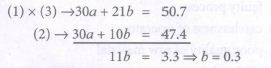
Substituting b = 0.3 in (2) we get
30a + 3 = 47.4 ⇒ 30a = 44.4
\(a=\frac{44.4}{30}=1.48\)
∴ The straight line trend is y = 1.48x + 0.3

12th Standard Syllabus & Materials
12th Standard
TN 12th Computer Applications களப்பெயர் முறைமை (DNS) Sample Question Papers Study Material - QB365 Set A
NEW12th Standard
TN 12th Computer Applications வலையமைப்பு எடுத்துக்காட்டுகள் மற்றும் நெறிமுறைகள் Sample Question Papers Study Material - QB365 Set A
NEW12th Standard
TN 12th Computer Applications கணினி வலையமைப்பு ஓர் அறிமுகம் Sample Question Papers Study Material - QB365 Set A
NEW12th Standard
TN 12th Computer Applications PHP-உடன் MySQL-ஐ இணைத்தல் Sample Question Papers Study Material - QB365 Set A



Tamilnadu Stateboard 12th Standard Subjects

Maths

Chemistry

Physics

Biology

Computer Science
Business Maths and Statistics

Economics

Commerce

Accountancy

History

Computer Applications
Biology
Computer Technology
Computer Applications
Computer Science
Business Maths and Statistics
Commerce
Economics
Maths
Chemistry
Physics
Computer Technology
History
Accountancy

Tamil

English

French
Tamilnadu Stateboard Standards
