
 100% FREE ACCESS
12th Standard Syllabus & Materials
12th Standard
TN 12th Computer Applications மின்னணு தரவு பரிமாற்றம் Sample Question Papers Study Material - QB365 Set A
NEW12th Standard
TN 12th Computer Applications மின் - வணிக பாதுகாப்பு அமைப்புகள் Sample Question Papers Study Material - QB365 Set A
NEW12th Standard
TN 12th Computer Applications மின்னணு செலுத்தல் முறைகள் Sample Question Papers Study Material - QB365 Set A
NEW12th Standard
TN 12th Computer Applications மின் - வணிகம் Sample Question Papers Study Material - QB365 Set A
NEW12th Standard
TN 12th Computer Applications திறந்த மூல கருத்துருக்கள் Sample Question Papers Study Material - QB365 Set A
NEW12th Standard
TN 12th Computer Applications வலையமைப்பு வடமிடல் Sample Question Papers Study Material - QB365 Set A

Published on: 03/09/2022
QB365 provides a detailed and simple solution for every Possible Book Back Questions in Class 12 Business Maths Subject - Applied Statistics, English Medium. It will help Students to get more practice questions, Students can Practice these question papers in addition to score best marks.
Download Tamil Nadu 12th Standard Business Maths and Statistics question papers, model tests, one-mark questions, important questions, and public exam papers in PDF format. Free study materials and answer keys for TN State Board students.
Questions + Answers key
Take MCQ Business Maths and Statistics Test
1.
The following are the sample means and ranges for 10 samples, each of size 5. Calculate the control limits for the mean chart and range chart and state whether the process is in control or not.
| Sample number | 1 | 2 | 3 | 4 | 5 | 6 | 7 | 8 | 9 | 10 |
| Mean | 5.10 | 4.98 | 5.02 | 4.96 | 4.96 | 5.04 | 4.94 | 4.92 | 4.92 | 4.98 |
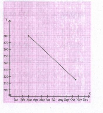
| Range | 0.3 | 0.4 | 0.2 | 0.4 | 0.1 | 0.1 | 0.8 | 0.5 | 0.3 | 0.5 |
2.
The following data gives the average life(in hours) and range of 12 samples of 5 lamps each. The data are
| Sample No | 1 | 2 | 3 | 4 | 5 | 6 |
| Sample Mean | 1080 | 1390 | 1460 | 1380 | 1230 | 1370 |
| Sample Range | 410 | 670 | 180 | 320 | 690 | 450 |
| Sample No | 7 | 8 | 9 | 10 | 11 | 12 |
| Sample Mean | 1310 | 1630 | 1580 | 1510 | 1270 | 1200 |
| Sample Range | 380 | 350 | 270 | 660 | 440 | 310 |
Construct control charts for mean and range. Comment on the control limits.
3.
From the following data, calculate the control limits for the mean and range chart.
| Sample No. | 1 | 2 | 3 | 4 | 5 | 6 | 7 | 8 | 9 | 10 |
| Sample Observations | 50 | 51 | 50 | 48 | 46 | 55 | 45 | 50 | 47 | 56 |
| 55 | 50 | 53 | 53 | 50 | 51 | 48 | 56 | 53 | 53 | |
| 52 | 53 | 48 | 50 | 44 | 56 | 53 | 54 | 49 | 55 | |
| 49 | 50 | 52 | 51 | 48 | 47 | 48 | 53 | 52 | 54 | |
| 54 | 46 | 47 | 53 | 47 | 51 | 51 | 57 | 54 | 52 |
4.
Using the following data, construct Fisher’s Ideal Index Number and Show that it satisfies Factor Reversal Test and Time Reversal Test?
| Commodities | Price | Quantity | ||
| Base Year | Current year | Base Year | Current year | |
| Wheat | 6 | 10 | 50 | 56 |
| Ghee | 2 | 2 | 100 | 120 |
| Firewood | 4 | 6 | 60 | 60 |
| Sugar | 10 | 12 | 30 | 24 |
| Cloth | 8 | 12 | 40 | 36 |
5.
Calculate the Laspeyre’s, Paasche’s and Fisher’s price index number for the following data. Interpret on the data.
| Commodities | Base Year | Current Year | ||
| Price | Quantity | Price | Quantity | |
| A | 170 | 562 | 72 | 632 |
| B | 192 | 535 | 70 | 756 |
| C | 195 | 639 | 95 | 926 |
| D | 187 | 128 | 92 | 255 |
| E | 185 | 542 | 92 | 632 |
| F | 150 | 217 | 180 | 314 |
| 7 | 12.6 | 12.7 | 12.5 | 12.8 |
| 8 | 12.4 | 12.3 | 12.6 | 12.5 |
| 9 | 12.6 | 12.5 | 12.3 | 12.6 |
| 10 | 12.1 | 12.7 | 12.5 | 12.8 |
6.
Fit a straight line trend by the method of least squares to the following data.
| Year | 1980 | 1981 | 1982 | 1983 | 1984 | 1985 | 1986 | 1987 |
| Sales | 50.3 | 52.7 | 49.3 | 57.3 | 56.8 | 60.7 | 62.1 | 58.7 |
7.
In a certain bottling industry the quality control inspector recorded the weight of each of the 5 bottles selected at random during each hour of four hours in the morning.
| Time | Weights in ml | ||||
| 8:00 AM | 43 | 41 | 42 | 43 | 41 |
| 9:00 AM | 40 | 39 | 40 | 39 | 44 |
| 10:00 AM | 42 | 42 | 43 | 38 | 40 |
| 11:00 AM | 39 | 43 | 40 | 39 | 42 |
8.
In a production process, eight samples of size 4 are collected and their means and ranges are given below. Construct mean chart and range chart with control limits.
| Sample number | 1 | 2 | 3 | 4 | 5 | 6 | 7 | 8 |
| \(\overset{-}{X}\) | 12 | 13 | 11 | 12 | 14 | 13 | 16 | 15 |
| R | 2 | 5 | 4 | 2 | 3 | 2 | 4 | 3 |
9.
The following data show the values of sample means and the ranges for ten samples of size 4 each. Construct the control chart for mean and range chart and determine whether the process is in control
| Sample number | 1 | 2 | 3 | 4 | 5 | 6 | 7 | 8 | 9 | 10 |
| \(\overset{-}{X}\) | 29 | 26 | 37 | 34 | 14 | 45 | 39 | 20 | 34 | 23 |
| R | 39 | 10 | 39 | 17 | 12 | 20 | 05 | 21 | 23 | 15 |
10.
A quality control inspector has taken ten samples of size four packets each from a potato chips company. The contents of the sample are given below, Calculate the control limits for mean and range chart.
| Sample Number | Observations | |||
| 1 | 2 | 3 | 4 | |
| 1 | 12.5 | 12.3 | 12.6 | 12.7 |
| 2 | 12.8 | 12.4 | 12.4 | 12.8 |
| 3 | 12.1 | 12.6 | 12.5 | 12.4 |
| 4 | 12.2 | 12.6 | 12.5 | 12.3 |
| 5 | 12.4 | 12.5 | 12.5 | 12.5 |
| 6 | 12.3 | 12.4 | 12.6 | 12.6 |
| 7 | 12.6 | 12.7 | 12.5 | 12.8 |
| 8 | 12.4 | 12.3 | 12.6 | 12.5 |
| 9 | 12.6 | 12.5 | 12.3 | 12.6 |
| 10 | 12.1 | 12.7 | 12.5 | 12.8 |
(Given for n = 5, A2 = 0.58, D3 = 0 and D4 = 2.115)
11.
The following data show the values of sample mean (\(\overset{-}{X}\)) and its range (R) for the samples of size five each. Calculate the values for control limits for mean, range chart and determine whether the process is in control.
| Sample number | 1 | 2 | 3 | 4 | 5 | 6 | 7 | 8 | 9 | 10 |
| Mean | 11.2 | 11.8 | 10.8 | 11.6 | 11.0 | 9.6 | 10.4 | 9.6 | 10.6 | 10.0 |
| Range | 7 | 4 | 8 | 5 | 7 | 4 | 8 | 4 | 7 | 9 |
( conversion factors for n = 5, A2 = 0.58, D3 = 0 and D4 = 2.115)
12.
Construc \(\overset {-}{X}\) and R charts for the following data:
| Sample Number | Observations | ||
| 1 | 32 | 36 | 42 |
| 2 | 28 | 32 | 40 |
| 3 | 39 | 52 | 28 |
| 4 | 50 | 42 | 31 |
| 5 | 42 | 45 | 34 |
| 6 | 50 | 29 | 21 |
| 7 | 44 | 52 | 35 |
| 8 | 22 | 35 | 44 |
( Given for n = 3, A2 = 0.58,D3 = 0 and D4 = 2.115)
13.
Ten samples each of size five are drawn at regular intervals from a manufacturing process. The sample means ( \(\overset{-}{X}\) ) and their ranges (R ) are given below:
| Sample number | 1 | 2 | 3 | 4 | 5 | 6 | 7 | 8 | 9 | 10 |
| \(\overset {-}{X}\) | 49 | 45 | 48 | 53 | 39 | 47 | 46 | 39 | 51 | 45 |
| R | 7 | 5 | 7 | 9 | 5 | 8 | 8 | 6 | 7 | 6 |
Calculate the control limits in respect of \(\overset {-}{X}\) chart. (Given A2 = 0.58, D3 = and D4 = 2.115) Comment on the state of control.
14.
A machine is set to deliver packets of a given weight. Ten samples of size five each were recorded. Below are given relevant data:
| Sample number | 1 | 2 | 3 | 4 | 5 | 6 | 7 | 8 | 9 | 10 |
| \(\overset {-}{X}\) | 15 | 17 | 15 | 18 | 17 | 14 | 18 | 15 | 17 | 16 |
| R | 7 | 7 | 4 | 9 | 8 | 7 | 12 | 4 | 11 | 5 |
Calculate the control limits for mean chart and the range chart and then comment on the state of control. (conversion factors for n = 5, A2 = 0.58, D3 = 0 and D4 = 2.115
15.
Calculate Fisher’s index number to the following data. Also show that it satisfies Time Reversal Test.
| Commodity | Price in Rupees per unit | Number of units | ||
| Price (Rs.) | Quantity (Kg) | Price (Rs.) | Quantity (Kg) | |
| Food | 40 | 12 | 65 | 14 |
| Fuel | 72 | 14 | 78 | 20 |
| Clothing | 36 | 10 | 36 | 15 |
| Wheat | 20 | 6 | 42 | 4 |
| Others | 46 | 8 | 52 | 6 |
16.
Using Fisher’s Ideal Formula, compute price index number for 1999 with 1996 as base year, given the following:
| Year | Commodity: A | Commodity: B | Commodity: C | |||
| Price (Rs.) | Quantity (Kg) | Price (Rs.) | Quantity (Kg) | Price (Rs.) | Quantity (Kg) | |
| 1996 | 5 | 10 | 8 | 6 | 6 | 3 |
| 1999 | 4 | 12 | 7 | 7 | 5 | 4 |
17.
Using the following data, construct Fisher’s Ideal index and show how it satisfies Factor Reversal Test and Time Reversal Test?
| Commodity | Price in Rupees per unit | Number of units | ||
| Base year | Current year | Base year | Current year | |
| A | 6 | 10 | 50 | 56 |
| B | 2 | 2 | 100 | 120 |
| C | 4 | 6 | 60 | 60 |
| D | 10 | 12 | 50 | 24 |
| E | 8 | 12 | 40 | 36 |
18.
Compute
(i) Laspeyre’s
(ii) Paasche’s
(iii) Fisher’s Index numbers for the 2010 from the following data.
| Commodity | Price | Quantity | ||
| 2000 | 2010 | 2000 | 2010 | |
| A | 12 | 14 | 18 | 16 |
| B | 15 | 16 | 20 | 15 |
| C | 14 | 15 | 24 | 20 |
| D | 12 | 12 | 29 | 23 |
19.
Calculate price index number for 2005 by
(a) Laspeyre’s
(b) Paasche’s method
| Commodity | 1995 | 2005 | ||
| Price | Quantity | Price | Quantity | |
| A | 5 | 60 | 15 | 70 |
| B | 4 | 20 | 8 | 35 |
| C | 3 | 15 | 6 | 20 |
20.
The following table shows the number of salesmen working for a certain concern:
| Year | 1992 | 1993 | 1994 | 1995 | 1996 |
| No. of salesmen | 46 | 48 | 42 | 56 | 52 |
Use the method of least squares to fit a straight line and estimate the number of salesmen in 1997.
21.
Calculate the seasonal indices from the following data using the average from the following data using the average method:
| I Quarter | II Quarter | III Quarter | IV Quarter | |
| 2008 | 72 | 68 | 62 | 76 |
| 2009 | 78 | 74 | 78 | 72 |
| 2010 | 74 | 70 | 72 | 76 |
| 2011 | 76 | 74 | 74 | 72 |
| 2012 | 72 | 72 | 76 | 68 |
22.
Use the method of monthly averages to find the monthly indices for the following data of production of a commodity for the years 2002, 2003 and 2004.
| 2002 | 15 | 18 | 17 | 19 | 16 | 20 | 21 | 18 | 17 | 15 | 14 | 18 |
| 2003 | 20 | 18 | 16 | 13 | 12 | 15 | 22 | 16 | 18 | 20 | 17 | 15 |
| 2004 | 18 | 25 | 21 | 11 | 14 | 16 | 19 | 20 | 17 | 16 | 18 | 20 |
23.
The sales of a commodity in tones varied from January 2010 to December 2010 as follows:
| In year 2010 | Jan | Feb | Mar | Apr | May | Jun | Jul | Aug | Sep | Oct | Nov | Dec |
| Sales (in tones) | 280 | 240 | 270 | 300 | 280 | 290 | 210 | 200 | 230 | 200 | 230 | 210 |
Fit a trend line by the method of semi-average.
24.
Determine the equation of a straight line which best fits the following data
| Year | 2000 | 2001 | 2002 | 2003 | 2004 |
| Sales(Rs.000) | 35 | 36 | 79 | 80 | 40 |
Compute the trend values for all years from 2000 to 2004
25.
The annual production of a commodity is given as follows :
\(\begin{array}{|c|c|} \hline \text { Year } & \text { Production (in tones) } \\ \hline 1995 & 155 \\ \hline 1996 & 162 \\ \hline 1997 & 171 \\ \hline 1998 & 182 \\ \hline 1999 & 158 \\ \hline 2000 & 180 \\ \hline 2001 & 178 \\ \hline \end{array}\)
Fit a straight line trend by the method of least squares.
26.
Compute the average seasonal movement for the following series
| Year | Quarterly Production | |||
| I | II | III | IV | |
| 2002 | 3.5 | 3.8 | 3.7 | 3.5 |
| 2003 | 3.6 | 4.2 | 3.4 | 4.1 |
| 2004 | 3.4 | 3.9 | 3.7 | 4.2 |
| 2005 | 4.2 | 4.5 | 3.8 | 4.4 |
| 2006 | 3.9 | 4.4 | 4.2 | 4.6 |
27.
You are given below the values of sample mean ( \(\bar{X}\) ) and the range ( R ) for ten samples of size 5 each. Draw mean chart and comment on the state of control of the process.
| Sample number | 1 | 2 | 3 | 4 | 5 | 6 | 7 | 8 | 9 | 10 |
| \(\overset{-}{X}\) | 43 | 49 | 37 | 44 | 45 | 37 | 51 | 46 | 43 | 47 |
| R | 5 | 6 | 5 | 7 | 7 | 4 | 8 | 6 | 4 | 6 |
Given the following control chart constraint for : n = 5, A2 = 0.58, D3 = 0 and D4 = 2.115
28.
The following data gives readings of 10 samples of size 6 each in the production of a certain product. Draw control chart for mean and range with its control limits.
| Sample | 1 | 2 | 3 | 4 | 5 | 6 | 7 | 8 | 9 | 10 |
| Mean | 383 | 508 | 505 | 582 | 557 | 337 | 514 | 614 | 707 | 753 |
| Range | 95 | 128 | 100 | 91 | 68 | 65 | 148 | 28 | 37 | 80 |
29.
The data shows the sample mean and range for 10 samples for size 5 each. Find the control limits for mean chart and range chart.
| Sample | 1 | 2 | 3 | 4 | 5 | 6 | 7 | 8 | 9 | 10 |
| Mean | 21 | 26 | 23 | 18 | 19 | 15 | 14 | 20 | 16 | 10 |
| Range | 5 | 6 | 9 | 7 | 4 | 6 | 8 | 9 | 4 | 7 |
30.
31.
Calculate the cost of living index number by consumer price index number for the year 2016 with respect to base year 2011 of the following data
\(\begin{array}{|c|c|c|c|} \hline & {\text { Price }} & \\ \begin{array}{c} \text { Commodities } \\ \text { } \end{array} & \begin{array}{c} \text { Base } \\ \text { year } \end{array} & \begin{array}{c} \text { Current } \\ \text { year } \end{array} & \text { Quantity } \\ \hline \text { Rice } & 32 & 48 & 25 \\ \hline \text { Sugar } & 25 & 42 & 10 \\ \hline \text { Oil } & 54 & 85 & 6 \\ \hline \text { Coffee } & 250 & 460 & 1 \\ \hline \text { Tea } & 175 & 275 & 2 \\ \hline \end{array}\)
32.
Calculate the cost of living index number for the year 2015 with respect to base year 2010 of the following data.
\(\begin{array}{|c|c|c|c|} \hline \text { Commodities } & \begin{array}{c} \text { Number of } \\ \text { Units (2010) } \end{array} & \begin{array}{c} \text { Price } \\ (2010) \end{array} & \begin{array}{c} \text { Price } \\ (2015) \end{array} \\ \hline \text { Rice } & 5 & 1500 & 1750 \\ \hline \text { Sugar } & 3.5 & 1100 & 1200 \\ \hline \text { Pulses } & 3 & 800 & 950 \\ \hline \text { Cloth } & 2 & 1200 & 1550 \\ \hline \text { Ghee } & 0.75 & 550 & 700 \\ \hline \text { Rent } & 12 & 2500 & 3000 \\ \hline \text { Fuel } & 8 & 750 & 600 \\ \hline \text { Misc } & 10 & 3200 & 3500 \\ \hline \end{array}\)
33.
Calculate the cost of living index number for the following data.
| Commodities | Quantity 2005 |
Price | |
| 2005 | 2010 | ||
| A | 10 | 7 | 9 |
| B | 12 | 6 | 8 |
| C | 17 | 10 | 15 |
| D | 19 | 14 | 16 |
| E | 15 | 12 | 17 |
34.
Construct Fisher’s price index number and prove that it satisfies both Time Reversal Test and Factor Reversal Test for data following data.
| Commodities | Base Year | Current Year | ||
| Price | Quantity | Price | Quantity | |
| Rice | 40 | 5 | 48 | 4 |
| Wheat | 45 | 2 | 42 | 3 |
| Rent | 90 | 4 | 95 | 6 |
| Fuel | 85 | 3 | 80 | 2 |
| Transport | 50 | 5 | 65 | 8 |
| Miscellaneous | 65 | 1 | 72 | 3 |
35.
Calculate Fisher’s price index number and show that it satisfies both Time Reversal Test and Factor Reversal Test for data given below.
| Commodities | Base Year | Current Year | ||
| Price | Quantity | Price | Quantity | |
| Rice | 10 | 5 | 11 | 6 |
| Wheat | 12 | 6 | 13 | 4 |
| Rent | 14 | 8 | 15 | 7 |
| Fuel | 16 | 9 | 17 | 8 |
| Transport | 18 | 7 | 19 | 5 |
| Miscellaneous | 20 | 4 | 21 | 3 |
36.
Calculate Fisher’s price index number and show that it satisfies both Time Reversal Test and Factor Reversal Test for data given below.
| Commodities | Price | Quandity | ||
| 2003 | 2009 | 2003 | 2009 | |
| Rice | 10 | 13 | 4 | 6 |
| Wheat | 125 | 18 | 7 | 8 |
| Rent | 25 | 29 | 5 | 9 |
| Fuel | 11 | 14 | 8 | 10 |
| Miscellaneous | 14 | 17 | 6 | 7 |
37.
Construct the Laspeyre’s, Paasche’s and Fisher’s price index number for the following data. Comment on the result.
| Commodities | Base Year | Current Year | ||
| Price | Quantity | Price | Quantity | |
| Rice | 15 | 5 | 16 | 8 |
| Wheat | 10 | 6 | 18 | 9 |
| Rent | 8 | 7 | 15 | 8 |
| Fuel | 9 | 5 | 12 | 6 |
| Transport | 11 | 4 | 11 | 7 |
| Miscellaneous | 16 | 6 | 15 | 10 |
38.
the Laspeyre’s, Paasche’s and Fisher’s price index number for the following data. Interpret on the data.
| Commodities | Price | Quandity | ||
| 2000 | 2010 | 2000 | 2010 | |
| Rice | 38 | 35 | 6 | 7 |
| Wheat | 12 | 18 | 7 | 10 |
| Rent | 10 | 15 | 10 | 15 |
| Fuel | 25 | 30 | 12 | 16 |
| Miscellaneous | 30 | 33 | 8 | 10 |
39.
Calculate the seasonal index for the quarterly production of a product using the method of simple averages.
| Year | I Quarter | II Quarter | III Quarter | IV Quarter |
| 2005 | 255 | 351 | 425 | 400 |
| 2006 | 269 | 310 | 396 | 410 |
| 2007 | 291 | 332 | 358 | 395 |
| 2008 | 198 | 289 | 310 | 357 |
| 2009 | 200 | 290 | 331 | 359 |
| 2010 | 250 | 300 | 350 | 400 |
40.
41.
Given below are the data relating to the sales of a product in a district.
Fit a straight line trend by the method of least squares and tabulate the trend values.
| Year | 1995 | 1996 | 1997 | 1998 | 1999 | 2000 | 2001 | 2002 |
| Sales | 6.7 | 5.3 | 4.3 | 6.1 | 5.6 | 7.9 | 5.8 | 6.1 |
42.
Given below are the data relating to the production of sugarcane in a district.
Fit a straight line trend by the method of least squares and tabulate the trend values.
| Year | 2000 | 2001 | 2002 | 2003 | 2004 | 2005 | 2006 |
| Prod.of Sugarcane | 40 | 45 | 46 | 42 | 47 | 50 | 46 |
1.
\(\overline {\overline{X}} = \frac {5.10+4.98+5.02+4.96+4.96+5.04+4.94+4.92+4.92+4.98}{10}\)
\(\overline {\overline{X}}\) = \(\frac {49.82}{10} = 4.982\)
\(\overline {\overline{R}} = \frac {0.3+.4+.2+.4+.1+.1+.8+.5+.3+.5}{10}\)
\(\overline {R}\) = \(\frac {3.6}{10}\) = 0.36
The control limits of mean chart are
UCL = \(\overline {\overline{X}} + A_{2} \overline{R}\)
= 4.982 + .577(.36)
= 4.982+ .208 = 5.19
CL = 4.982
LCL = \(\overline {\overline{X}} - A_{2} \overline{R}\)
= 4.982 - .208 = 4.774
The control limits of R-chart are
UCL = D4\(\overline {R}\) = 2.114 (.36) = 0.761
CL = \(\overline {R}\) = .36
LCL = D3\(\overline {R}\) = 0
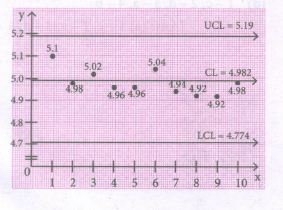
Mean Chart
Range chart
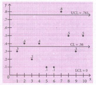
Conclusion: The above diagram shows all the control lines with the data points plotted.
Since one in Range chart, lie outside the control limits, we can say that the process is out of control.
2.
\(\overline {\overline{X}} = \frac {1080+1390+1460+1380+1230+1370+1310+1630+1580+1510+1270+1200}{12}\)
\(\overline {\overline{X}}\) = \(\frac {16410}{12}\) = 1367.5
\(\overline {\overline{R}} = \frac {410+670+180+320+690+450+380+350+270+660+440+310}{12}\)
\(\overline {R}\) = \(\frac {5130}{12}\) = 427.5
The control limits of mean chart are
UCL = \(\overline {\overline{X}} + A_{2} \overline{R}\)
= 1367.5 + 0.577(427.5)
= 1367.5 + 246.67 = 1614.17
CL = \(\overline {\overline{X}}\) = 1367.5
LCL = \(\overline {\overline{X}} - A_{2} \overline{R}\)
= 1367.5 - 246.67 = 1120.83
The control limits of range chart are
UCL = D4\(\overline {R}\) = 2.114 (427.5) = 903.74
CL = \(\overline {R}\) = 427.5
[For n=5, A2 = 0.577, D3 = 0, D4 = 2.114]
LCL = D3\(\overline {R}\) = 0
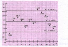
\(\overline {X}\) - chart

R-chart
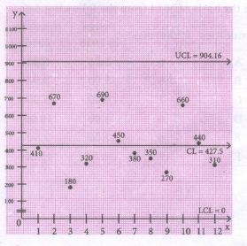
Conclusion: The above diagram shows all the control lines with the data points plotted.
Since one point in mean chart, lie outside the control limits, we can say that the process is out of control.
3.
| Sample No. | Observation | Total | x | R = Xmax - Xmin | ||||
| 1 | 2 | 3 | 4 | 5 | ||||
| 1 | 50 | 55 | 52 | 49 | 54 | 260 | 52 | 55-49 = 6 |
| 2 | 51 | 50 | 53 | 50 | 46 | 250 | 50 | 53-46 = 7 |
| 3 | 50 | 53 | 48 | 52 | 47 | 250 | 50 | 53-47 = 6 |
| 4 | 48 | 53 | 50 | 51 | 53 | 255 | 51 | 53-48 = 5 |
| 5 | 46 | 50 | 44 | 48 | 47 | 235 | 47 | 50-44 = 6 |
| 6 | 55 | 51 | 56 | 47 | 51 | 260 | 52 | 56-47=9 |
| 7 | 45 | 48 | 53 | 48 | 51 | 245 | 49 | 53-45=8 |
| 8 | 50 | 56 | 54 | 53 | 57 | 270 | 54 | 57-50 = 7 |
| 9 | 47 | 53 | 49 | 52 | 54 | 255 | 51 | 54-47 = 7 |
| 10 | 56 | 53 | 55 | 54 | 52 | 270 | 54 | 56-52 = 4 |
| 510 | 65 | |||||||
\(\overline {\overline{X}}\) = \(\frac {510}{10}\) = 51
\(\overline {R}\) = \(\frac {65}{10}\) = 6.5
The control limits of mean chart are
UCL = \(\overline {\overline{X}} + A_{2} \overline{R}\)
= 51 + 0.577 (6.5)
= 51 + 3.75 = 57.75
CL = \(\overline {\overline{X}}\) = 51
LCL = \(\overline {\overline{X}} - A_{2} \overline{R}\)
= 51 - 3.75 = 47.25
The control limits of range chart are
UCL = D4\(\overline {R}\) = 2.114 (6.3) = 13.32
CL = \(\overline {R}\) = 6.5
[For n=5, A2 = 0.577, D3 = 0, D4 = 2.114]
LCL = D3\(\overline {R}\) = 0
4.
| Commodities | Price | Quantity | ||
| Base year (p0) | Current year (p1) | q0 | q1 | |
| Wheat | 6 | 10 | 50 | 56 |
| Ghee | 2 | 2 | 60 | 60 |
| Firewood | 4 | 6 | 60 | 60 |
| Sugar | 10 | 12 | 30 | 24 |
| Cloth | 8 | 12 | 40 | 36 |
| p0q0 | p1q1 | p0q1 | p1q0 |
| 300 | 560 | 336 | 500 |
| 200 | 240 | 240 | 200 |
| 240 | 360 | 240 | 360 |
| 300 | 288 | 240 | 360 |
| 320 | 432 | 288 | 480 |
| 1360 | 1880 | 1344 | 1900 |
Fisher's price index number
\(P^{F}_{01}\) = \(\sqrt{ \frac {\sum p_{1}q_{0}}{\sum p_{0}q_{0}} \times \frac{ {\sum p_{1}q_{1}} }{{\sum p_{0}q_{1}}}{}}\times 100\)
= \(\sqrt\frac {1900 \times 1880}{1360 \times 1344} \times 100\)
= \(\sqrt\frac {3572000}{1827840} \times 100\)
= \(\sqrt {1.954} \times 100\)
\(P^{F}_{01}\) = 139.8
Time reversal test:
\(P _{01} \times P_{10}\) = \(\sqrt{ \frac {\sum p_{1}q_{0}\times \sum p_{1}q_{1}\times \sum p_{0}q_{1}\times \sum p_{0}q_{0}}{\sum p_{0}q_{0}\times \sum p_{0}q_{1}\times \sum p_{1}q_{1} \times \sum p_{1}q_{0}} }\)
= 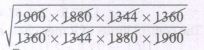
= \(\sqrt {1}\) = 1
∴ \(P _{01} \times P_{10}\) = 1
Factor reversal test:
\(P _{01} \times Q_{01}\) = \(\sqrt{ \frac {\sum p_{1}q_{0}\times \sum p_{1}q_{1}\times \sum q_{1}p_{0}\times \sum q_{1}p_{1}}{\sum p_{0}q_{0}\times \sum p_{0}q_{1}\times \sum q_{0}p_{0} \times \sum q_{0}p_{1}} }\)
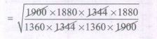
= \(\frac {1880}{1360} = \frac {\sum p_{1}q_{1}}{\sum p_{0}q_{0}}\)
Hence, it satisfies time reversal test and factor reversal test.
5.
| Commodities | Base year | Current year | ||
| p0 | q0 | p1 | q1 | |
| A | 170 | 562 | 72 | 632 |
| B | 192 | 535 | 70 | 756 |
| C | 195 | 639 | 95 | 926 |
| D | 187 | 128 | 92 | 255 |
| E | 185 | 542 | 92 | 632 |
| F | 150 | 217 | 180 | 314 |
| 7 | 12.6 | 12.7 | 12.5 | 12.8 |
| 8 | 12.4 | 12.3 | 12.6 | 12.5 |
| 9 | 12.6 | 12.5 | 12.3 | 12.6 |
| 10 | 12.1 | 12.7 | 12.5 | 12.8 |
| p0q0 | p1q1 | p0q1 | p1q0 |
| 95540 | 45504 | 107440 | 40464 |
| 102750 | 52920 | 145152 | 37450 |
| 124605 | 87970 | 180570 | 60705 |
| 100270 | 58144 | 116920 | 49864 |
| 32550 | 56520 | 47100 | 39060 |
| 160.02 | 160 | 161.28 | 158.75 |
| 152.52 | 157.5 | 155 | 154.98 |
| 157.5 | 154.98 | 158.76 | 153.75 |
| 153.67 | 160 | 154.88 | 158.75 |
| 480244.7 | 325150.48 | 645496.92 | 239945.23 |
Laspeyre's pnce index number
\(P^{L}_{01}\) = \(\frac {\sum p_{1}q_{0}}{\sum p_{0}q_{0}} \times 100\)
= \(\frac {239945.23}{480244.71} \times 100 \)
Paasches index number
\(P^{p}_{01}\) = \(\frac {\sum p_{1}q_{0}}{\sum p_{0}q_{0}} \times 100\)
= \(\frac {325150.48}{645496.92} \times 100 \)
= 50.37
Fisher's index number
\(P^{F}_{01}\) = \(\sqrt{ \frac {\sum p_{0}q_{0}}{\sum p_{0}q_{0}} \times \frac{ {\sum p_{0}q_{0}} }{{\sum p_{0}q_{0}}}{}}\times 100\)
= \(\sqrt\frac {239945.23 \times 325150.48}{480244.71 \times 645496.92} \times 100\)
= \(\sqrt\frac {489.84 \times 570.22}{693 \times 803.43} \times 100\)
= 50.1
6.
| Year X | Sales Y | X = \(\frac {x-1983.5}{0.5}\) | XY | X2 |
| 1980 | 50.3 | -7 | -352.1 | 49 |
| 1981 | 52.7 | -5 | -263.5 | 25 |
| 1982 | 49.3 | -3 | -147.9 | 9 |
| 1983 | 57.3 | -1 | -57.3 | 1 |
| 1984 | 56.8 | 1 | 56.8 | 1 |
| 1985 | 60.7 | 3 | 182.1 | 9 |
| 1986 | 62.1 | 5 | 310.5 | 25 |
| 1987 | 58.7 | 7 | 410.9 | 49 |
| 447.9 | 0 | 139.5 | 168 |
Since \(\sum X = 0, a = \frac {\sum Y}{n} = \frac {447.9}{8} = 55.9875\)
b = \(\frac {\sum XY}{\sum X^{2}} = \frac{139.5}{168}\) = 0.83035
∴ The straight line trend is obtained by
Y = a + bX ⇒ Y = 55.9875 + 0.830 \((\frac {x-1983.5}{0.5})\)
= 55.9875 + 0.8304 (-5)
= 55.9875 - 4.152
= 51.8355
7.
| Time | Weight in ml | Total | \(\overline {X}\) | R = x max - xmin | ||||
| 1 | 2 | 3 | 4 | 5 | ||||
| 8.00 AM | 43 | 41 | 42 | 43 | 41 | 210 | \(\frac {210}{5} = 42\) | 43-41 = 2 |
| 9:00 AM | 40 | 39 | 40 | 39 | 44 | 202 | \(\frac {202}{5} = 40.4\) | 43-41 = 2 |
| 10.00 AM | 42 | 42 | 43 | 38 | 40 | 205 | \(\frac {205}{5} = 41\) | 43-38 = 5 |
| 11:00 AM | 39 | 43 | 40 | 39 | 42 | 203 | \(\frac {203}{5} = 40.6\) | 43-39 = 4 |
| 164 | 16 | |||||||
\(\overline {\overline{X}}\) = \(\frac {164}{4}\) = 41
\(\overline {R}\) = \(\frac {16}{4}\) = 4
Control limits for \(\overline {X}\) - chart
UCL = \(\overline {\overline{X}} + A_{2} \overline {R}\)
= 41 + 0.577 (4)
= 41 + 2.308 = 43.31
CL = \(\overline {\overline{X}} \) = 41
[when n = 5, A2= 0.577, D3 = 0, D4 = 2.114]
LCL = \(\overline {\overline{X}} - A_{2} \overline {R}\)
= 41 - 2.308 = 38.69
The control limits of R-chart are
UCL = D4 \(\overline{R}\) = 2.114 (4) = 8.44
CL = \(\overline{R}\) = 4
LCL = D3 \(\overline{R}=0\)
8.
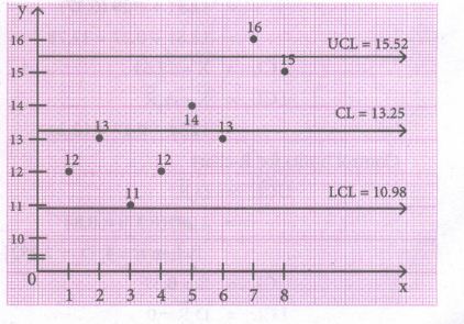
\(\overline {\overline {X}} = \frac{12+13+11+12+14+13+16+15}{8}\) = \(\frac {106}{8}\) = 13.25
\(\overline{R}\) = \( \frac{2+5+4+2+3+2+4+3}{8}\)
\(\overline{R}\) = \(\frac {25}{8}\) = 3.12
Control limits for mean chart
UCL = \(\overline {\overline{X}} + A_{2} \overline {R}\)
= 13.25+.729(3.12)
= 13.25+2.27 = 15.52
CL = \(\overline {\overline{X}}\) = 13.25
LCL = \(\overline {\overline{X}} - A_{2} \overline {R}\)
= 13.25-2.27 =10.98
Control limits.for R-chart
UCL = D4\(\overline {R}\) = 2.282 = (3.12)
= 7.12
CL = \(\overline {R}\) = 3.12
LCL = D3\(\overline {R}\) = 0
Mean (\(\overline {X}\)) chart
R chart
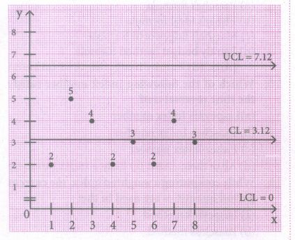
Conclusion: The above diagram shows all the control lines with the data points plotted.
Since one point in X - chart, lie out of the control lines, we can say that the process is out of control.
9.
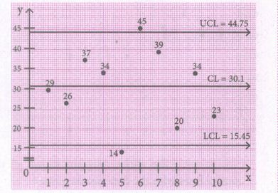
\(\overline {\overline {X}} = \frac{29+26+37+34+14+45+39+20+34+23}{10}\) = \(\frac {301}{10}\) = 30.1
\(\overline{R}\) = \( \frac{39+10+39+17+12+20+5+21+23+15}{10}\)
\(\overline{R}\) = \(\frac {201}{10}\) = 20.1
Control limits for mean chart
UCL = \(\overline {\overline{X}} + A_{2} \overline {R}\)
= 30.1+.729(20.1)
= 30.1 + 14.65 = 44.75
CL = \(\overline {\overline{X}}\) = 30.1
LCL = \(\overline {\overline{X}} - A_{2} \overline {R}\)
= 30.1 - 14.65 =15.45
Control limits.for R-chart
UCL = D4\(\overline {R}\) = 2.282 = (20.1)
= 45.86
CL = \(\overline {R}\) = 20.1
LCL = D3 \(\overline {R}\) = 0
Mean (\(\overline {X}\)) chart
Mean (\(\overline {R}\)) chart
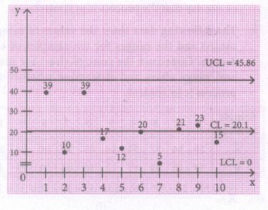
Conclusion: The above diagram shows all the control lines with the data points plotted.
Since one point in \(\overline {X}\) - chart, lie out of the control lines, we can say that the process is out of control.
10.
| Sample No | Observations | Total | \(\overline {X}\) | R = x max - xmin | |||
| 1 | 2 | 3 | 4 | ||||
| 1 | 12.5 | 12.3 | 12.6 | 12.7 | 50.1 | \(\frac {50.1}{4} = 12.5\) | 12.7-12.3 = 0.4 |
| 2 | 12.8 | 12.4 | 12.4 | 12.8 | 50.4 | \(\frac {50.4}{4} = 12.6\) | 12.8-12.4 = 0.4 |
| 3 | 12.1 | 12.6 | 12.5 | 12.4 | 49.6 | \(\frac {49.6}{4} = 12.4\) | 12.6-12.1 = 0.5 |
| 4 | 12.2 | 12.6 | 12.5 | 12.3 | 49.6 | \(\frac {49.6}{4} = 12.4\) | 12.6-12.2 = 0.4 |
| 5 | 12.4 | 12.5 | 12.5 | 12.5 | 49.9 | \(\frac {49.9}{4} = 12.5\) | 12.6-12.4 = 0.1 |
| 6 | 12.3 | 12.4 | 12.6 | 12.6 | 49.9 | \(\frac {49.9}{4} = 12.5\) | 12.6-12.3 = 0.3 |
| 7 | 12.6 | 12.7 | 12.5 | 12.8 | 50.6 | \(\frac {50.6}{4} = 12.7\) | 12.6-12.5 = 0.3 |
| 8 | 12.4 | 12.3 | 12.6 | 12.5 | 49.8 | \(\frac {49.8}{4} = 12.5\) | 12.6-12.3 =.3 |
| 9 | 12.6 | 12.5 | 12.3 | 12.6 | 50 | \(\frac {50}{4} = 12.5\) | 12.6-12.3 =.3 |
| 10 | 12.1 | 12.7 | 12.5 | 12.8 | 50.1 | \(\frac {50.1}{4} = 12.5\) |
12.8-12.1 =.7 |
| 125.1 | 3.7 | ||||||
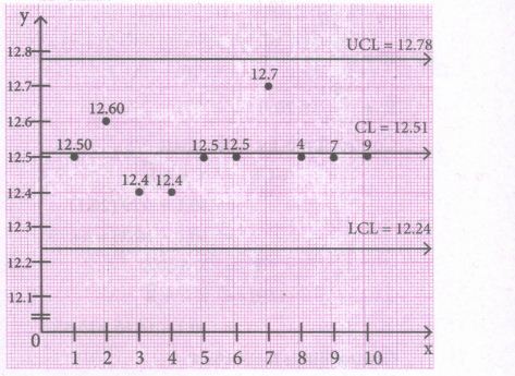
\(\overline {\overline{X}} = \frac {125.1}{10}\) = 12.51
\(\overline{R} = \frac {3.7}{10}\) = 0.37
Control limits for \(\overline {X}\) - chart
UCL = \(\overline {\overline{X}} + A_{2} \overline {R}\)
= [when n = 4, A2 = .729]
= 12.51 + .729 (0.37)
= 12.51 + 0.27 = 12.78
CL = \(\overline {\overline{X}}\) = 12.51
LCL = \(\overline {\overline{X}} - A_{2} \overline {R}\)
= 12.51 - 0.27 = 12.24
Control limits for R-chart
UCL = D4 \(\overline{R}\)
= 2.282(0.37) = 0.84
[when n = 4, D4 = 2.282]
CL = \(\overline{R}\) = 0.37
LCL = D3 \(\overline{R}\) = 0
[When n = 4, D3 = 0]
\(\overline {X}\) - chart
\(\overline {R}\) - chart
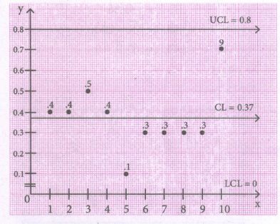
Conclusion: The above diagram shows all the control lines with the data points plotted.
Since all the points lie within the control limits, we can say that the process is in control.
11.
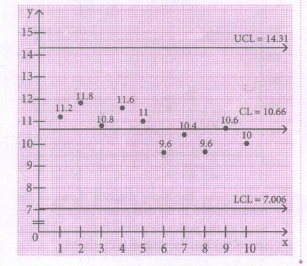
\(\overline {\overline {X}} = \frac{11.2+ 11.8+ 10.8+ 11.6+ 11.0+ 9.6+ 10.4+9.6+ 10.6+ 10}{10}\) = \(\frac {106.6}{10}\) = 10.66
\(\overline {\overline {R}} = \frac{7+4+8+5+7+4+8+4+7+9}{10}\) = \(\frac {63}{10}\) = 6.3
Control limits for \(\overline {X}\) - chart
UCL = \(\overline {\overline{X}} + A_{2} \overline {R}\)
= 10.66 + 0.58 (6.3)
= 10.66 + 3.654 = 14.31
CL = \(\overline {\overline {X}}\) = 10.66
LCL = \(\overline {\overline{X}} - A_{2} \overline {R}\)
= 10.66 - 3.654 = 7.006
Control limits for R-chart
UCL = D4\(\overline {R}\) = 2.115(6.3) = 13.3
CL = \(\overline {R}\) = 6.3
LCL = D3\(\overline {R}\) = 0
Mean (\(\overline {X}\)) chart
R chart
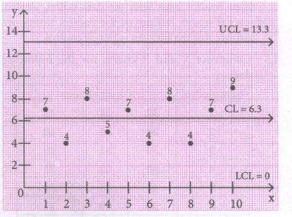
Conclusion: The above diagram shows all the control lines with the data points plotted. Since all the points lie within the control limits, we can say that the process is in control.
12.
| Sample No | Observations | Total | \(\overline {X}\) | R = x max - xmin | ||
| 1 | 2 | 3 | ||||
| 1 | 32 | 36 | 42 | 110 | \(\frac {100}{3} = 36.7\) | 42-32 = 10 |
| 2 | 28 | 32 | 40 | 100 | \(\frac {100}{3} = 33.3\) | 40-28 = 12 |
| 3 | 39 | 52 | 28 | 119 | \(\frac {119}{3} = 39.7\) | 52 -28 = 24 |
| 4 | 50 | 42 | 31 | 123 | \(\frac {123}{3} = 41\) | 50-31 = 19 |
| 5 | 42 | 45 | 34 | 121 | \(\frac {123}{3} = 40.3\) | 45-34 = 29 |
| 6 | 50 | 29 | 21 | 100 | \(\frac {100}{3} = 33.3\) | 50-21 = 29 |
| 7 | 44 | 52 | 35 | 131 | \(\frac {131}{3} = 43.7\) | 52-35 = 17 |
| 8 | 22 | 35 | 44 | 101 | \(\frac {101}{3} = 33.7\) | 44-22 = 22 |
| 301.7 | 144 | |||||
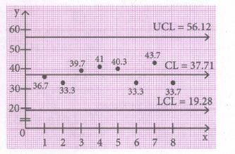
\(\overline {\overline{X}}\) = \(\frac {301.7}{8}\) = 37.71
\(\overline{R}\) = \(\frac {144}{8}\) = 18
Control limits for \(\overline {X}\) - chart
UCl = \(\overline {\overline{X}} + A_{2} \overline {R}\)
= 37.71 + 0.58 (18)
= 37.71 + 18.44
[when n = 3, A2 = 1.023]
UCL = 56.12
CL = \(\overline {\overline{X}}\) = 37.71
LCL = \(\overline {\overline{X}} - A_{2} \overline {R}\)
= 37.71 - 18.44
LCL = 19.28
Control limits for R-chart
UCL = D4 \(\overline {R}\) = 2.2574(18) = 46.33
CL = \(\overline {R}\) = 18
LC = D3 \(\overline {R}\) = 0
when n = 3, D4 = 2.574]
\(\overline {X}\) - chart
.\(\overline {R}\) - chart
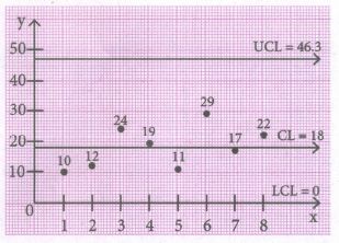
Conclusion: The above diagram shows all the control lines with the data points plotted. Since all the points lie within the control limits, we can say that the process is in control.
13.
\(\begin{array}{|c|c|c|c|c|c|c|c|c|c|c|c|} \hline \text { Sample number } & 1 & 2 & 3 & 4 & 5 & 6 & 7 & 8 & 9 & 10 & \text { Total } \\ \hline \bar{X} & 49 & 45 & 48 & 53 & 39 & 47 & 46 & 39 & 51 & 45 & 462 \\ \hline \mathbf{R} & 7 & 5 & 7 & 9 & 5 & 8 & 8 & 6 & 7 & 6 & 68 \\ \hline \end{array}\)
\(\overline{\bar{X}}=\frac{\sum \bar{X}}{10}=\frac{462}{10}=46.2 \)
\(\bar{R}=\frac{\sum R}{10}=\frac{68}{10}=6.8 \)
\(\text { The control limits for } \overline{\mathrm{X}} \text { chart is }\)
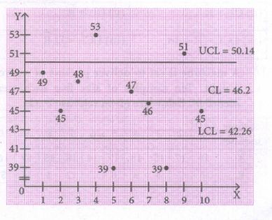
\(\mathrm{UCL}=\overline{\overline{\mathrm{X}}}+\mathrm{A}_{2} \overline{\mathrm{R}}=46.2+(0.58)(6.8)=50.14\)
\(\mathrm{CL}=46.2\)
\(\mathrm{LCL}=\overline{\mathrm{X}}-\mathrm{A}_{2} \overline{\mathrm{R}}=46.2-(0.58)(6.8)=42.26 \)
The control limits for range chart is
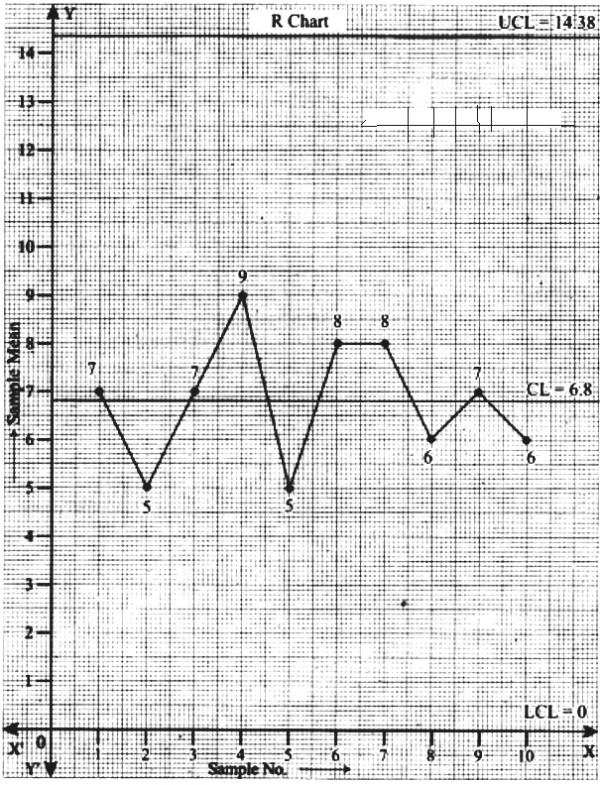
\(\mathrm{UCL}=\mathrm{D}_{4} \overline{\mathrm{R}}=(2.115)(6.8)=14.38 \)
\(\mathrm{CL}=\overline{\mathrm{R}}=6.8 \)
\(\mathrm{LCL}=\mathrm{D}_{3} \overline{\mathrm{R}}=0(6.8)=0\)
From the \(\overline X\) chart, we see that 4 points are outside the control limit lines. So we say that the process is out of control.
Conclusion: The above diagram shows all the three control lines with the data points plotted, since 2 points fall out of the control limits, we can say that the process is out of control.
14.
| Sample No | \(\overline {X}\) | R |
| 1 | 15 | 7 |
| 2 | 17 | 7 |
| 3 | 15 | 4 |
| 4 | 18 | 9 |
| 5 | 17 | 8 |
| 6 | 14 | 7 |
| 7 | 18 | 12 |
| 8 | 15 | 4 |
| 9 | 17 | 11 |
| 10 | 16 | 5 |
\(\overline {\overline {X}} = \frac{15+17+15+18+17+14+18+15+17+15+17+16}{10}\) = \(\frac {162}{10}\) = 16.2
\(\overline {R}\) = \(\frac{7 + 7 + 4+ 9+ 8+ 12 + 7 + 4+ 11+ 15}{10}\) = \(\frac {74}{10}\) = 7.4
Control limits for mean chart
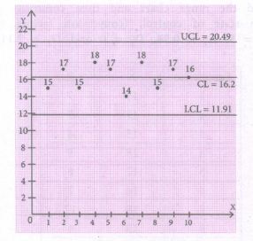
UCL = \(\overline {\overline{X}} + A_{2} \overline {R}\)
= 16.2 + 0.58(7.4)
= 16.2 + 4.292 = 20.492
[∴ A2 = 0.58]
CL = \(\overline {\overline{X}}\) = 16.2
LCL = \(\overline {\overline{X}} - A_{2} \overline {R}\)
= 16.2 - 0.58(7.4)
= 16.2 - 4.292 = 11.91
Control limits for R-chart
UCL = D4 \(\overline{R}\)
= 2.115 (7.4) = 15.65
[∴ D4 = 2.115]
CL = \(\overline{R}\) = 7.4
LCL = D3 \(\overline{R}\)
= 0(\(\overline{R}\)) = 0
[∴ D3 = 0]
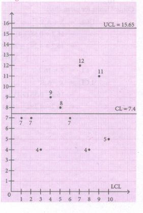
Conclusion : The above diagram shows all the control lines with the data points plotted. Since all the points lie within the control limits, we can say that the process is in control.
15.
| Commodity | 2016 | 2017 | ||
| p0 | q0 | p1 | q1 | |
| Food | 40 | 12 | 65 | 14 |
| Fuel | 72 | 14 | 78 | 20 |
| Clothing | 36 | 10 | 36 | 15 |
| Wheat | 20 | 6 | 42 | 4 |
| Others | 46 | 8 | 52 | 6 |
| p0q0 | p1q1 | p1q0 | p0q1 |
| 480 | 910 | 780 | 560 |
| 1008 | 1560 | 1092 | 1440 |
| 120 | 168 | 252 | 80 |
| 368 | 312 | 416 | 276 |
| 2336 | 3490 | 2900 | 2896 |
Fisher's price index number
\(P^{F}_{01}\) = \(\sqrt \frac {\sum p_{1}q_{0}\times \sum p_{1}q_{1}}{{\sum p_{0}q_{0}\times \sum p_{0}q_{1}}}\) × 100
= \(\sqrt \frac {2900\times3490}{2336\times2896} \times 100\)
= \(\sqrt \frac{10121000}{6765056} \times{100}\)
= \(\sqrt{1.496}\times{100}\)
\(P^{F}_{01}\) = 122.31
Time Reversal Test
P01 × P10 = \(\sqrt \frac {\sum p_{1}q_{0}\times \sum p_{1}q_{1}\times{\sum p_{0}q_{1}\times \sum p_{0}q_{0}}}{{\sum p_{0}q_{0}\times \sum p_{0}q_{1}\times \sum p_{1}q_{1}\times \sum p_{1}q_{0}}}\)
= \(\sqrt \frac {2900\times3490\times{2896\times2336}}{2336\times2896\times3490\times2900}\)
= \(\sqrt {1}\) = 1
Hence, it satisfies time reversal test.
16.
| Commodity | p0 | p1 | q0 | q1 |
| A | 5 | 4 | 10 | 12 |
| B | 8 | 7 | 6 | 7 |
| C | 6 | 5 | 3 | 4 |
| p0q0 | p0q1 | p1q0 | p1q1 |
| 50 | 60 | 40 | 48 |
| 48 | 56 | 42 | 49 |
| 18 | 24 | 15 | 20 |
| 116 | 140 | 97 | 117 |
Fisher's price index number
\(P^{F}_{01}\) = \(\sqrt \frac {\sum p_{1}q_{0}\times \sum p_{1}q_{1}}{{\sum p_{0}q_{0}\times \sum p_{0}q_{1}}}\) × 100
= \(\sqrt \frac {97\times117}{116\times140} \times 100\)
= \(\sqrt \frac {11349}{16240} \times 100\)
= \(\sqrt {0.6988}\times100\)
\(P^{F}_{01}\) = 83.59
17.
| Commodity | Price in Rupees per unit | Number of units | ||
| p0 | p1 | q0 | q1 | |
| A | 6 | 10 | 50 | 56 |
| B | 2 | 2 | 100 | 120 |
| C | 4 | 6 | 60 | 60 |
| D | 10 | 12 | 50 | 24 |
| E | 8 | 12 | 40 | 36 |
| p0q0 | p0q1 | p1q0 | p1q1 |
| 300 | 560 | 500 | 336 |
| 200 | 240 | 200 | 240 |
| 240 | 360 | 360 | 240 |
| 500 | 288 | 600 | 240 |
| 320 | 432 | 480 | 288 |
| 1560 | 1880 | 2140 | 1344 |
Fisher's price index number
\(P^{P}_{01}\) = \(\sqrt \frac {\sum p_{1}q_{0}\times \sum p_{1}q_{1}}{{\sum p_{0}q_{0}\times \sum p_{0}q_{1}}}\) × 100
= \(\sqrt \frac{2140\times1880}{1560\times1344} \times 100\)
= \(\sqrt \frac{4023200}{2096640} \times 100\)
= \(\sqrt {1.9188} \times 100\)
\(P^{F}_{01}\) = 138.5
Time reversal test :
P01 × P10 = \(\sqrt \frac{\sum p_{1}q_{0}\times{p_{1}q_{1}}\times{p_{0}q_{1}}\times{p_{0}q_{0}}}{{\sum p_{0}q_{0}\times{p_{0}q_{1}}\times{p_{1}q_{1}}\times{p_{1}q_{0}}}}\)
= \(\sqrt \frac{2140\times1880 \times 1344\times1560}{1560\times1344 \times 1880\times2140 }\)
= \(\sqrt 1\) = 1
Time reversal test = 1
Factor reversal test:
P01 × Q 01 = \(\sqrt \frac{\sum p_{1}q_{0}\times{p_{1}q_{1}}\times{p_{0}q_{1}}\times{p_{0}q_{0}}}{{\sum p_{0}q_{0}\times{p_{0}q_{1}}\times{p_{1}q_{1}}\times{p_{1}q_{0}}}}\)
\(=\sqrt \frac{2140\times1880 \times 1344\times1560}{1560\times1344 \times 1880\times2140 }\)
= \(\sqrt{(\frac{1880}{1560})^2}\)
= \(\frac {1880}{1560}\)
P01 × Q01 = \({\frac {\sum p_{1}q_{1}}{\sum p_{0}q_{0}}}\)
18.
| Commodity | Price | Quantity | ||
| 2000 (p0) | 2010 (p1) | 2000 (q0) | 2010 (q1) | |
| A | 12 | 14 | 18 | 16 |
| B | 15 | 16 | 20 | 15 |
| C | 14 | 15 | 24 | 20 |
| D | 12 | 12 | 29 | 23 |
| p0q0 | p0q1 | p1q0 | p1q1 |
| 216 | 192 | 252 | 224 |
| 300 | 225 | 320 | 240 |
| 336 | 280 | 360 | 300 |
| 348 | 276 | 348 | 276 |
| 1200 | 973 | 1280 | 1040 |
(i) Laspeyre's index number
\(P^{L}_{01}\) = \({\frac {\sum p_{1}q_{0}}{\sum p_{0}q_{0}}} \times 100\)
= \(\frac {1280}{1200} \times {100}\) = 106.66
(ii) Paasches index number
\(P^{P}_{01}\) = \({\frac {\sum p_{1}q_{1}}{\sum p_{0}q_{1}}} \times 100\)
= \(\frac {1040}{973} \times {100}\) = 106.88
(iii) Fisher's index number
\(P^{F}_{01}\) = \(\sqrt \frac {\sum p_{1}q_{0}\times \sum p_{1}q_{1}}{{\sum p_{0}q_{0}\times \sum p_{0}q_{1}}}\) × 100
= \(\sqrt \frac{1280\times1040}{1200\times973} \times 100\)
=\(\sqrt \frac {1331200}{1167600} \times {100}\)
= \(\sqrt {1.1401} \times {100}\)
= 1.067 × 100
\(P^{F}_{01}\) = 106.7
19.
| Commodity | 1995 | 2005 | ||
| Price(p0) | (q0) | Price | Quantity | |
| A | 5 | 60 | 15 | 70 |
| B | 4 | 20 | 8 | 35 |
| C | 3 | 15 | 6 | 20 |
| p0q0 | p0q1 | p1q0 | p1q1 |
| 300 | 350 | 900 | 1050 |
| 80 | 140 | 160 | 280 |
| 45 | 60 | 90 | 120 |
| 425 | 550 | 1150 | 1450 |
Laspeyre's price index number
\(P^{L}_{01}\) = \({\frac {\sum p_{1}q_{0}}{\sum p_{0}q_{0}}} \times 100\)
= \(\frac {1150}{425} \times {100}\) = 270.58
Paasche's index number
\(P^{L}_{01}\) = \({\frac {\sum p_{1}q_{0}}{\sum p_{0}q_{1}}} \times 100\)
= \(\frac {1450}{550} \times {100}\) = 263.63
20.
| Year (X) | No. of Salesmen Y | X = x -1994 | X2 | XY |
| 1992 | 46 | -2 | 4 | -92 |
| 1993 | 48 | -1 | 1 | -48 |
| 1994 | 42 | 0 | 0 | 0 |
| 1995 | 56 | 1 | 1 | 56 |
| 1996 | 52 | 2 | 4 | 104 |
| 244 | 0 | 10 | 20 |
Smce \(\sum\)X = 0, a =\(\frac {\sum Y}{n}\) = \(\frac {244}{5}\) = 48.8
b = \(\frac {\sum XY}{\sum X^2}\) = \(\frac {20}{10}\) = 2
∴ The required equation of the straight line trend is given by
Y = a + bX \(\Rightarrow \) Y = 48.8 + 2X
\(\Rightarrow \) Y = 48.8 +2 (X - 1994) .... (1)
∴ Number of salesmen in 1997 is put X = 1997 in (1)
∴ Y = 48.8 + 2 (1997 - 1994)
= 48.8 + 2 (3)
= 48.8 + 6 = 54.8
∴ Number of salesmen in 1997 is 54.8
21.
| Year | I Quarter | II Quarter | III Quarter | IV Quarter |
| 2008 | 72 | 68 | 62 | 76 |
| 2009 | 78 | 74 | 78 | 72 |
| 2010 | 74 | 70 | 72 | 76 |
| 2011 | 76 | 74 | 74 | 72 |
| 2012 | 72 | 72 | 76 | 68 |
| Total | 372 | 358 | 362 | 364 |
| Average | 74.4 | 71.6 | 72.4 | 72.8 |
Grand average = \(\frac {74.4+ 71.6+ 72.4 + 72.8}{4}\) = \(\frac {291.2}{4}\) = 72.8
S.I for I Quarter = \(\frac {Average \ for \ I \ Quarter}{Grand \ average}\) × 100
= \(\frac {74.4}{72.8}\) × 100 = 102.19
S.I for II Quarter = \(\frac {71.6}{72.8}\) × 100 = 98.35
S.I for III Quarter = \(\frac {72.4}{72.8}\) × 100 = 99.45
S.I for IV Quarter = \(\frac {72.8}{72.8}\) × 100 = 100
22.
| Year | Jan | Feb | Mar | Apr | May | Jun | Jul | Aug | Sep | Oct | Nov | Dec |
| 2002 | 15 | 18 | 17 | 19 | 16 | 20 | 21 | 18 | 17 | 15 | 14 | 18 |
| 2003 | 20 | 18 | 16 | 13 | 12 | 15 | 22 | 16 | 18 | 20 | 17 | 15 |
| 2004 | 18 | 25 | 21 | 11 | 14 | 16 | 19 | 20 | 17 | 16 | 18 | 20 |
| Monthly Total | 53 | 61 | 54 | 43 | 42 | 51 | 62 | 54 | 52 | 51 | 49 | 53 |
| Monthly Average | 17.6 | 20.3 | 18 | 14.3 | 14 | 17 | 20.6 | 18 | 17.3 | 17 | 16.3 | 17.6 |
Grand Average = \(= \frac {17.6+ 20.3+ 18+ 14.3 + 14+ 17 + 20.6+ 18+ 17.3 + 17 + 16.3+ 17.6}{12}\) = \(\frac {208}{12}\) = 17.33
S.I for Jan = \(\frac {17.6}{17.33}\) × 100 = 101.56
S.I for Feb = \(\frac {20.3}{17.33}\) × 100 = 117.14
S.I for Mar = \(\frac {18}{17.33}\) × 100 = 103.87
S.I for April = \(\frac {14.3}{17.33}\) × 100 = 82.51
S.I for May = \(\frac {14}{17.33}\) × 100 = 80.78
S.I for June = \(\frac {17}{17.33}\) × 100 = 98.10
S.I for July = \(\frac {20}{17.33}\) × 100 = 118.87
S.I for Aug = \(\frac {20.6}{17.33}\) × 100 = 103.87
S.I for Sep = \(\frac {17.3}{17.33}\) × 100 = 99.83
S.I for Oct = \(\frac {17}{17.33}\) × 100 = 98.10
S.I for Nov = \(\frac {16.3}{17.33}\) × 100 = 94.06
S.I for Dec = \(\frac {17.6}{17.33}\) × 100 = 101.56
23.
| Year 2010 | Sales (in tones) |
|---|---|
| Jan | 280 |
| Feb | 240 |
| Mar | 270 |
| Apr | 300 |
| May | 280 |
| June | 290 |
Average
\(\frac {280 + 240 + 270 + 300 + 280 + 290}{6}\) = \(\frac {1660}{6}\) = 276.6666
| Year 2010 | Sales (in tones) |
|---|---|
| Jul | 210 |
| Aug | 200 |
| Sep | 230 |
| Oct | 200 |
| Nov | 230 |
| Dec | 210 |
\(\frac {210+ 200+ 230+ 200+ 230+ 210}{6}\) = \(\frac {1280}{6}\) = 213.333
Since the number of years is even (12), we can equally divide the given data into two equal parts and obtain the averages of first 6 months and last 6 months.
24.
| Year | Sales | X=x- 2002 | X2 | XY |
| 2000 | 35 | -2 | 4 | -70 |
| 2001 | 36 | -1 | 1 | -36 |
| 2002 | 79 | 0 | 0 | 0 |
| 2003 | 80 | 1 | 1 | 80 |
| 2004 | 40 | 2 | 4 | 80 |
| 270 | 0 | 10 | 54 |
Since \(\sum X = 0, a = \frac{\sum Y}{n}\) = \(\frac {270}{5}\) = 54
b = \(\frac {\sum XY}{\sum X^2} = \frac {54}{10}\) = 5.4
∴ The required equation of the straight line trend is given by Y = a +bX
\(\Rightarrow \) Y = 54 + 5.4 (x - 2002)
The trend values can be obtained as follows:
When X = 2000, Yt = 54 + 5.4 (2000 - 2002)
= 54 + 5.4 (-2) = 43.2
When X = 2001, Yt = 54 + 5.4 (2001 - 2002)
= 54 + 5.4(-1) = 48.6
When X = 2002, Yt = 54 + 5.4 (2002 - 2002)
= 54
When X = 2003, Yt = 54 + 5.4 (2003 - 2002)
= 54 + 5.4 = 59.4
When X = 2004, Yt = 54 + 5.4 (2004 - 2002)
= 54 + 5.4 (2) = 64.8
25.
| Year X | Production in tonnes (Y) | X = x-1998 | X2 | XY |
| 1995 | 155 | -3 | 9 | -465 |
| 1996 | 162 | -2 | 4 | -324 |
| 1997 | 171 | -1 | 1 | -171 |
| 1998 | 182 | 0 | 0 | 0 |
| 1999 | 158 | 1 | 1 | 158 |
| 2000 | 180 | 2 | 4 | 360 |
| 20001 | 178 | 3 | 9 | 534 |
| 1186 | 0 | 28 | 92 |
Since \(\sum\)X = 0, a = \(\frac {\sum Y}{n}\) = \(\frac {1186}{7}\) = 169.428.
b = \(\frac {\sum XY}{\sum X^2}\) \(\frac {92}{28}\) = 3.285
∴ The required equation of the straight line trend is given by Y = a + bX
\(\Rightarrow \) Y= 69.428 + 3.285 (x - 1998)
26.
| Year | Quarterly production | |||
| I | II | III | IV | |
| 2002 | 3.5 | 3.8 | 3.7 | 3.5 |
| 2003 | 3.6 | 4.2 | 3.4 | 4.1 |
| 2004 | 3.4 | 3.9 | 3.7 | 4.2 |
| 2005 | 4.2 | 4.5 | 3.8 | 4.4 |
| 2006 | 3.9 | 4.4 | 18.8 | 20.8 |
| Quarterly Total | 18.6 | 20.8 | 18.8 | 20.8 |
| Average | 3.72 | 4.16 | 3.76 | 20.8 |
Grand average = (3.72 + 4.16 + 3.76 + 4.16)/4 = 3.95
Seasonal Index (S.I) for I quarter = (Average of I quarter)/(Grand Average) \(\times\) 100
S.I. for I quarter = 3.72/3.95 \(\times\) 100 = 94.1772
S.I. for II quarter = 4.16/3.95 \(\times\) 100 = 105.3165
S.I. for III quarter = 3.76/3.95 \(\times\) 100 = 95.1899
S.I. for IV quarter = 4.16/3.95 \(\times\) 100 = 105.3165
Thus we obtain the average seasonal movement.
27.
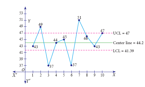
\(\overset { = }{ X } =\frac { \sum { \bar { X } } }{ 10 } =\frac { 442 }{ 10 } =44.2\)
\(\bar { R } =\frac { \sum { R } }{ n } =\frac { 58 }{ 10 } =5.8\)
\(UCL=\overset { = }{ X } +{ A }_{ 2 }\bar { R } \)
= 44.2 + 0.483(5.8) = 47.00
\(CL=\overset { = }{ X } =44.2\)
\(LCL=\overset { = }{ X } -{ A }_{ 2 }\bar { R } =44.2-0.483(5.8)=41.39\)
The above diagram shows all the three control lines with the data points plotted, since four points falls out of the control limits, we can say that the process is out of control.
28.
| Sample | 1 | 2 | 3 | 4 | 5 | 6 | 7 | 8 | 9 | 10 | Total |
| Mean | 383 | 508 | 505 | 582 | 557 | 337 | 514 | 614 | 707 | 753 | 5460 |
| Range | 95 | 128 | 100 | 91 | 68 | 65 | 148 | 28 | 37 | 80 | 840 |
\(\overset { = }{ X } =\frac { \sum { \bar { X } } }{ 10 } =\frac { 5460 }{ 10 } =546\)
The control limits for \(\overset{-}{X}\) chart is
\(UCL=\overset { = }{ X } +{ A }_{ 2 }\bar { R } =546+0.483(84)=586.57\)
\(CL=\overset { = }{ X } =546\)
\(LCL=\overset { = }{ X } -{ A }_{ 2 }\bar { R } =546-0.483(84)=505.43\)
\(\bar { R } =\frac { \sum { R } }{ n } =\frac { 840 }{ 10 } =84\)
The control limits for Range chart is
\(UCL={ D }_{ 4 }\bar { R } =2.004(84)=168.336\)
\(CL=\bar { R } =84\)
\(LCL={ D }_{ 3 }\bar { R } =0(84)=0\)
29.
| Sample | 1 | 2 | 3 | 4 | 5 | 6 | 7 | 8 | 9 | 10 | Total |
| Mean | 21 | 26 | 23 | 18 | 19 | 14 | 14 | 20 | 16 | 10 | 182 |
| Range | 5 | 6 | 9 | 7 | 4 | 6 | 8 | 9 | 4 | 7 | 65 |
\(\overset { = }{ X } =\frac { \sum { \overset { - }{ X } } }{ numberofsamples } =\frac { 182 }{ 10 } =18.2\quad \overset { - }{ R } =\frac { \sum { R } }{ n } =\frac { 65 }{ 10 } =6.5\)
The control limits for \(\overset{-}{X}\) chart is
\(UCL=\overset { = }{ X } +{ A }_{ 2 }\bar { R } =18.2+0.577(6.5)=21.95\)
\(CL=\overset { = }{ X } =18.2\)
\(LCL=\overset { = }{ X } -{ A }_{ 2 }\bar { R } =18.2-0.577(6.5)=14.5795\)
The control limits for Range chart is
\(UCL={ D }_{ 4 }\bar { R } =2.114(6.5)=13.741\)
\(CL=\bar { R } =65\)
\(LCL={ D }_{ 3 }\bar { R } =0(6.5)=0\)
30.
31.
Here the base year quantities are given, therefore we can apply Aggregate Expenditure Method.
| Commodities | Price | Quantity (q0) |
p0q0 | p1q0 | |
| Base year (P0) | Current year (P1) | ||||
| Rice | 32 | 48 | 25 | 800 | 1200 |
| Sugar | 25 | 42 | 10 | 250 | 420 |
| Oil | 54 | 85 | 6 | 324 | 510 |
| Coffe | 250 | 460 | 1 | 250 | 460 |
| Tea | 175 | 275 | 2 | 350 | 550 |
| Total | 1974 | 3140 | |||
Cost of Living Index Number=\(\frac { \sum { { p }_{ 1 }{ q }_{ 0 } } }{ \sum { { p }_{ 0 }{ q }_{ 0 } } } \times 100=\frac { 3140 }{ 1974 } \times 100 = 159.0679\)
Hence, the Cost of Living Index Number for a particular class of people for the year 2016 is increased by 59.0679 % as compared to the year 2011.
32.
Here the base year quantities are given, therefore we can apply Aggregate Expenditure Method.
| Commodities | Number of Units q0(2010) |
Price (2010) p0 |
Price (2015) p1 |
p0q0 | p1q0 |
| Rice | 5 | 1500 | 1750 | 7500 | 8750 |
| Sugar | 3.5 | 1100 | 1200 | 3850 | 4200 |
| Pulses | 3 | 800 | 950 | 2400 | 2850 |
| Cloth | 2 | 1200 | 1550 | 2400 | 3100 |
| Ghee | 0.75 | 550 | 700 | 412.5 | 525 |
| Rent | 12 | 2500 | 3000 | 30000 | 36000 |
| Fuel | 8 | 750 | 600 | 6000 | 4800 |
| Misc | 110 | 3200 | 3500 | 32000 | 35000 |
| Total | 84562.5 | 95225 |
Cost of Living Index Number \(=\frac { \sum { { p }_{ 1 }{ q }_{ 0 } } }{ \sum { { p }_{ 0 }{ q }_{ 0 } } } \times 100=\frac { 95225 }{ 84562.5 } \times 100=112.609\)
Hence, the Cost of Living Index Number for a particular class of people for the year 2015 is increased by 12.61 % as compared to the year 2010.
33.
| Commodities | Quantity 2005(Q0) |
Price | P1Q0 | P0Q0 | |
| 2005 (P0) |
2010 (P1) |
||||
| A | 10 | 7 | 9 | 90 | 70 |
| B | 12 | 6 | 8 | 96 | 72 |
| C | 17 | 10 | 15 | 255 | 170 |
| D | 19 | 14 | 16 | 304 | 266 |
| E | 15 | 12 | 17 | 255 | 180 |
| Total | 1000 | 758 | |||
Cost of Living Index Number
= \(\frac { \sum { { p }_{ 1 }{ q }_{ 0 } } }{ \sum { { p }_{ 0 }{ q }_{ 0 } } } \times 100=\frac { 1000 }{ 758 } \times 100=131.926 \)
34.
| Commodities | Base Year | Current Year | p0q0 | p0q1 | p1q0 | p1q1 | ||
| Price (p0) |
Quantity (q1) |
Price ((p0)) |
Quantity (q1) |
|||||
| Rice | 40 | 5 | 48 | 4 | 200 | 160 | 240 | 192 |
| Wheat | 45 | 2 | 42 | 3 | 90 | 135 | 84 | 126 |
| Rent | 90 | 4 | 95 | 6 | 360 | 540 | 380 | 570 |
| Fuel | 85 | 3 | 80 | 2 | 255 | 170 | 240 | 160 |
| Transport | 50 | 5 | 65 | 8 | 250 | 400 | 325 | 520 |
| Miscellaneous | 65 | 1 | 72 | 3 | 65 | 195 | 72 | 216 |
| Total | 1220 | 1600 | 1341 | 1784 | ||||
Fisher’s price index number
\({ P }_{ 01 }^{ F }=\left( \sqrt { \frac { \sum { { p }_{ 1 }{ q }_{ 10 } } \times \sum { { p }_{ 1 }{ q }_{ 1 } } }{ \sum { { p }_{ 0 }{ q }_{ 0 } } \times \sum { { p }_{ 0 }{ q }_{ 1 } } } } \right) \times 100=\left( \sqrt { \frac { 1341\times 1784 }{ 1220\times 1600 } } \right) \times 100=110.706\)
Time Reversal Test:P01x P10=1
\({ P }_{ 01 }\times { P }_{ 10 }=\sqrt { \left( \frac { \sum { { p }_{ 1 }{ q }_{ 0 } } \times \sum { { p }_{ 1 }{ q }_{ 1 } } \times \sum { { p }_{ 0 }{ q }_{ 1 } } \times \sum { { p }_{ 0 }{ q }_{ 0 } } }{ \sum { { p }_{ 0 }{ q }_{ 0 } } \times \sum { { p }_{ 0 }{ q }_{ 1 } } \times \sum { { p }_{ 1 }{ q }_{ 1 } } \times \sum { { p }_{ 1 }{ q }_{ 0 } } } \right) } \)
\({ P }_{ 01 }\times { P }_{ 10 }=\sqrt { \left( \frac { 1341\times 1784\times 1600\times 1220 }{ 1220\times 1600\times 1784\times 1341 } \right) } \)
P01x P10 = 1
Factor Reversal Test
\(P_{01} \times Q_{01}=\frac{\sum p_{1} q_{1}}{\sum p_{0} q_{0}}\)
\(P_{01} \times Q_{01}=\sqrt{\left(\frac{\sum p_{1} q_{0} \times \sum p_{1} q_{1} \times \sum q_{1} p_{0} \times \sum q_{1} p_{1}}{\sum p_{0} q_{0} \times \sum p_{0} q_{1} \times \sum q_{0} p_{0} \times \sum q_{0} p_{1}}\right)}\)
\(P_{01} \times Q_{01}=\sqrt{\left(\frac{1341 \times 1784 \times 1600 \times 1784}{1220 \times 1600 \times 1220 \times 1341}\right)}\)
\(P_{01} \times Q_{01}=\sqrt{\left(\frac{1784 \times 1784}{1220 \times 1220}\right)}=\frac{1784}{1220}\)
\(\Rightarrow P_{01} \times Q_{01}=\frac{\sum p_{1} q_{1}}{\sum p_{0} q_{0}}\)
35.
| Commodities | Base Year | Current Year | p0q0 | p0q1 | p1q0 | p1q1 | ||
| Price (p0) |
Quantity (q1) |
Price ((p0)) |
Quantity (q1) |
|||||
| Rice | 10 | 5 | 11 | 6 | 50 | 60 | 55 | 66 |
| Wheat | 12 | 6 | 13 | 4 | 72 | 48 | 78 | 52 |
| Rent | 14 | 8 | 15 | 7 | 112 | 98 | 120 | 105 |
| Fuel | 16 | 9 | 17 | 8 | 144 | 128 | 153 | 136 |
| Transport | 18 | 7 | 19 | 5 | 126 | 90 | 133 | 95 |
| Miscellaneous | 20 | 4 | 21 | 3 | 80 | 60 | 84 | 63 |
| Total | 584 | 484 | 623 | 517 | ||||
Fisher’s price index number
\({ P }_{ 01 }^{ F }=\left( \sqrt { \frac { \sum { { p }_{ 1 }{ q }_{ 10 } } \times \sum { { p }_{ 1 }{ q }_{ 1 } } }{ \sum { { p }_{ 0 }{ q }_{ 0 } } \times \sum { { p }_{ 0 }{ q }_{ 1 } } } } \right) \times 100=\left( \sqrt { \frac { 623\times 517 }{ 584\times 484 } } \right) \times 100=106.74\)
Time Reversal Test: P01 × P10 = 1
\({ P }_{ 01 }\times { P }_{ 10 }=\sqrt { \left( \frac { \sum { { p }_{ 1 }{ q }_{ 0 } } \times \sum { { p }_{ 1 }{ q }_{ 1 } } \times \sum { { p }_{ 0 }{ q }_{ 1 } } \times \sum { { p }_{ 0 }{ q }_{ 0 } } }{ \sum { { p }_{ 0 }{ q }_{ 0 } } \times \sum { { p }_{ 0 }{ q }_{ 1 } } \times \sum { { p }_{ 1 }{ q }_{ 1 } } \times \sum { { p }_{ 1 }{ q }_{ 0 } } } \right) } \)
\({ P }_{ 01 }\times { P }_{ 10 }=\sqrt { \left( \frac { 623\times 517\times 484\times 584 }{ 584\times 487\times 517\times 623 } \right) } \)
P01 x P10 = 1
Factor Reversal Test
\({ P }_{ 01 }\times { Q }_{ 01 }=\frac { \sum { { p }_{ 1 }{ q }_{ 1 } } }{ \sum { { p }_{ 0 }{ q }_{ 0 } } } \)
\({ P }_{ 01 }\times { P }_{ 01 }=\sqrt { \left( \frac { \sum { { p }_{ 1 }{ q }_{ 0 } } \times \sum { { p }_{ 1 }{ q }_{ 1 } } \times \sum { { p }_{ 1 }{ q }_{ 0 } } \times \sum { { p }_{ 1 }{ q }_{ 1 } } }{ \sum { { p }_{ 0 }{ q }_{ 0 } } \times \sum { { p }_{ 0 }{ q }_{ 1 } } \times \sum { { p }_{ 0 }{ q }_{ 0 } } \times \sum { { p }_{ 0 }{ q }_{ 1 } } } \right) } \)
\({ P }_{ 01 }\times { P }_{ 10 }=\sqrt { \left( \frac { 623\times 517\times 484\times 517 }{ 584\times 484\times 584\times 623 } \right) } \)
\({ P }_{ 01 }\times { P }_{ 01 }=\sqrt { \left( \frac { 517\times 517 }{ 585\times 584 } \right) } =\frac { 517 }{ 584 } \)
\({ P }_{ 01 }\times { P }_{ 01 }=\frac { \sum { { p }_{ 1 }{ q }_{ 1 } } }{ \sum { { p }_{ 0 }{ q }_{ 0 } } } \)
36.
| Commodities | Price | Quandity | p0q0 | p0q1 | p1q0 | p1q1 | ||
| 2003 (p0) |
2009 (q1) |
2003 (p0) |
2009 (q1) |
|||||
| Rice | 10 | 13 | 4 | 6 | 40 | 60 | 52 | 78 |
| Wheat | 125 | 18 | 7 | 8 | 105 | 120 | 126 | 144 |
| Rent | 25 | 29 | 5 | 9 | 125 | 225 | 145 | 261 |
| Fuel | 11 | 14 | 8 | 10 | 88 | 110 | 140 | 140 |
| Miscellaneous | 14 | 17 | 6 | 7 | 84 | 98 | 102 | 119 |
| Total | 442 | 613 | 537 | 742 | ||||
Fisher’s price index number
\({ P }_{ 01 }^{ F }=\left( \sqrt { \frac { \sum { { p }_{ 1 }{ q }_{ 10 } } \times \sum { { p }_{ 1 }{ q }_{ 1 } } }{ \sum { { p }_{ 0 }{ q }_{ 0 } } \times \sum { { p }_{ 0 }{ q }_{ 1 } } } } \right) \times 100=\left( \sqrt { \frac { 537\times 742 }{ 442\times 613 } } \right) \times 100=121.2684\)
Time Reversal Test:P01\(\times\) P10 = 1
\({ P }_{ 01 }\times { P }_{ 10 }=\sqrt { \left( \frac { \sum { { p }_{ 1 }{ q }_{ 0 } } \times \sum { { p }_{ 1 }{ q }_{ 1 } } \times \sum { { p }_{ 0 }{ q }_{ 1 } } \times \sum { { p }_{ 0 }{ q }_{ 0 } } }{ \sum { { p }_{ 0 }{ q }_{ 0 } } \times \sum { { p }_{ 0 }{ q }_{ 1 } } \times \sum { { p }_{ 1 }{ q }_{ 1 } } \times \sum { { p }_{ 1 }{ q }_{ 0 } } } \right) } \)
\({ P }_{ 01 }\times { P }_{ 10 }=\sqrt { \left( \frac { 537\times 742\times 613\times 442 }{ 442\times 613\times 742\times 537 } \right) } \)
\({ P }_{ 01 }\times { P }_{ 10 }=1\)
Factor Reversal Test
\({ P }_{ 01 }\times { Q }_{ 01 }=\frac { \sum { { p }_{ 1 }{ q }_{ 1 } } }{ \sum { { p }_{ 0 }{ q }_{ 0 } } } \)
\({ P }_{ 01 }\times { P }_{ 01 }=\sqrt { \left( \frac { \sum { { p }_{ 1 }{ q }_{ 0 } } \times \sum { { p }_{ 1 }{ q }_{ 1 } } \times \sum { { p }_{ 1 }{ q }_{ 0 } } \times \sum { { p }_{ 1 }{ q }_{ 1 } } }{ \sum { { p }_{ 0 }{ q }_{ 0 } } \times \sum { { p }_{ 0 }{ q }_{ 1 } } \times \sum { { p }_{ 0 }{ q }_{ 0 } } \times \sum { { p }_{ 0 }{ q }_{ 1 } } } \right) } \)
\({ P }_{ 01 }\times { P }_{ 01 }=\sqrt { \left( \frac { 537\times 742\times 613\times 742 }{ 442\times 613\times 442\times 537 } \right) } \)
\({ P }_{ 01 }\times { P }_{ 01 }=\sqrt { \left( \frac { 742\times 742 }{ 442\times 442 } \right) } =\frac { 742 }{ 442 } \Rightarrow { P }_{ 01 }\times { P }_{ 01 }=\frac { \sum { { p }_{ 1 }{ q }_{ 1 } } }{ \sum { { p }_{ 0 }{ q }_{ 0 } } } \)
37.
| Commodities | Base Year | Current Year | p0q0 | p0q1 | p1q0 | p1q1 | ||
| Price (p0) |
Quantity (q1) |
Price ((p0)) |
Quantity (q1) |
|||||
| Rice | 15 | 5 | 16 | 8 | 75 | 120 | 80 | 128 |
| Wheat | 10 | 6 | 18 | 9 | 60 | 90 | 108 | 162 |
| Rent | 8 | 7 | 15 | 8 | 56 | 64 | 105 | 120 |
| Fuel | 9 | 5 | 12 | 6 | 45 | 54 | 60 | 72 |
| Transport | 11 | 4 | 11 | 7 | 44 | 77 | 44 | 77 |
| Miscellaneous | 16 | 6 | 15 | 10 | 96 | 160 | 90 | 150 |
| Total | 376 | 565 | 487 | 709 | ||||
Laspeyre’s price index number
\({ P }_{ 01 }^{ L }=\frac { \sum { { p }_{ 1 }{ q }_{ 0 } } }{ \sum { { p }_{ 0 }{ q }_{ 0 } } } \times 100=\frac { 487}{ 376} \times 100=129.5212\)
Paasche’s price index number
\({ P }_{ 01 }^{ P }=\frac { \sum { { p }_{ 1 }{ q }_{ 1 } } }{ \sum { { p }_{ 0 }{ q }_{ 1 } } } \times 100=\frac { 709 }{ 565 } \times 100=125.4867\)
Fisher’s price index number
\({ P }_{ 01 }^{ F }=\sqrt { \frac { \sum { { p }_{ 1 }{ q }_{ 0 } } \times \sum { { p }_{ 1 }{ q }_{ 1 } } }{ \sum { { p }_{ 0 }{ q }_{ 0 } } \times \sum { { p }_{ 0 }{ q }_{ 1 } } } } \times 100=\sqrt { \frac { 487\times 709}{ 376\times 565} } \times 100=127.4879\)
On an average, there is an increase of 29.52%, 25.48% and 27.48% in the price of the commodities by Laspeyre’s, Paasche’s, Fisher’s price index number respectively, when the base year compared with the current year.
38.
| Commodities | Price | Quandity | p0q0 | p0q1 | p1q0 | p1q1 | ||
| 2000 (p0) |
2010 q1 |
2000 (p0) |
2010 (q1) |
|||||
| Rice | 38 | 35 | 6 | 7 | 228 | 266 | 210 | 245 |
| Wheat | 12 | 18 | 7 | 10 | 84 | 120 | 126 | 180 |
| Rent | 10 | 15 | 10 | 15 | 100 | 150 | 150 | 225 |
| Fuel | 25 | 30 | 12 | 16 | 300 | 400 | 630 | 480 |
| Miscellaneous | 30 | 33 | 8 | 10 | 240 | 300 | 264 | 330 |
| Total | 952 | 1236 | 1110 | 1460 | ||||
Laspeyre’s price index number
\({ P }_{ 01 }^{ L }=\frac { \sum { { p }_{ 1 }{ q }_{ 0 } } }{ \sum { { p }_{ 0 }{ q }_{ 0 } } } \times 100=\frac { 1110 }{ 952 } \times 100=116.60\)
On an average, there is an increase of 16.60 % in the price of the commodities when the year 2000 compared with the year 2010.
Paasche’s price index number
\({ P }_{ 01 }^{ P }=\frac { \sum { { p }_{ 1 }{ q }_{ 1 } } }{ \sum { { p }_{ 0 }{ q }_{ 1 } } } \times 100=\frac { 1460 }{ 1236 } \times 100=118.12\)
On an average, there is an increase of 18.12 % in the price of the commodities when the year 2000 compared with the year 2010.
Fisher’s price index number
\({ P }_{ 01 }^{ F }=\sqrt { \frac { \sum { { p }_{ 1 }{ q }_{ 0 } } \times \sum { { p }_{ 1 }{ q }_{ 1 } } }{ \sum { { p }_{ 0 }{ q }_{ 0 } } \times \sum { { p }_{ 0 }{ q }_{ 1 } } } } \times 100=\sqrt { \frac { 1110\times 1460 }{ 952\times 1236 } } \times 100=117.36\)
On an average, there is an increase of 17.36 % in the price of the commodities when the year 2000 compared with the year 2010.
39.
Computation of Seasonal Index by the method of simple averages.
| Year | I Quarter | II Quarter | III Quarter | IV Quarter |
| 2005 | 255 | 351 | 425 | 400 |
| 2006 | 269 | 310 | 396 | 410 |
| 2007 | 291 | 332 | 358 | 395 |
| 2008 | 198 | 289 | 310 | 357 |
| 2009 | 200 | 290 | 331 | 359 |
| 2010 | 250 | 300 | 350 | 400 |
| Quarterly Total |
1463 | 1872 | 2170 | 2321 |
| Quarterly Averages |
243.83 | 312 | 361.67 | 386.83 |
S.I for I Quarter = \(\frac{Average\ of \ I\ quarter }{Grand\ average} \times100\)
Grand Average = \(\frac{1304.333}{4}=326.0833\)
S.I for I Q = \(\frac{243.8333}{326.0833} \times100= 74.77;\)
S.I for II Q = \(\frac{312}{326.0833} \times100=95.68;\)
S.I for III Q = \(\frac{361.6667}{326.0833} \times 100=110.91; \)
S.I for IV Q = \(\frac{386.833}{326.0833} \times 100=118.63\)
40.
41.
Computation of trend values by the method of least squares.
In case of EVEN number of years, let us consider
\(X=\frac{\text{(x-Arithimetic mean of two middle years)}}{0.5}\)
| Year(x) | Sales(Y) | X=\(\frac{(x-1998.5)}{0.5}\) | XY | X2 | Trend Values (Yt) |
| 1995 | 6.7 | -7 | -46.9 | 49 | 5.6166 |
| 1996 | 5.3 | -5 | -26.5 | 25 | 5.7190 |
| 1997 | 4.3 | -3 | -12.9 | 9 | 5.8214 |
| 1998 | 6.1 | -1 | -6.1 | 1 | 5.9238 |
| 1999 | 5.6 | 1 | 5.6 | 1 | 6.0261 |
| 2000 | 7.9 | 3 | 23.7 | 9 | 6.1285 |
| 2001 | 5.8 | 5 | 29.0 | 25 | 6.2309 |
| 2002 | 6.1 | 7 | 42.7 | 49 | 6.3333 |
| N = 8 | 47.8 | \(\sum X\) = 0 | 8.6 | 168 |
\(a=\frac { \sum { Y } }{ n } =\frac { 47.8 }{ 8 } =5.975;\quad b=\frac { \sum { XY } }{ { \sum { X } }^{ 2 } } =\frac { 8.6 }{ 168 } =0.05119\)
Therefore, the required equation of the straight line trend is given by
Y = a + bX; Y = 5.975 + 0.05119 X.
When X = 1995, Yt = 5.975 + 0.05119\(\left( \frac { 1995-1998.5 }{ 0.5 } \right) =5.6166\)
When X = 1996, Yt = 5.975 + 0.05119\(\left( \frac { 1996-1998.5 }{ 0.5 } \right) =5.7190\)
similarly other values can be obtained.
42.
Computation of trend values by the method of least squares (ODD Years).
| Year(x) | Production of Sugarcane(Y) | X=(x–2003) | X2 | XY | Trend values(Yt) |
| 2000 | 40 | -3 | 9 | -120 | 42.04 |
| 2001 | 45 | -2 | 4 | -90 | 43.07 |
| 2002 | 46 | -1 | 1 | -46 | 44.11 |
| 2003 | 42 | 0 | 0 | 0 | 45.14 |
| 2004 | 47 | 1 | 1 | 47 | 46.18 |
| 2005 | 50 | 2 | 4 | 100 | 47.22 |
| 2006 | 46 | 3 | 9 | 138 | 48.25 |
| N=7 | \(\sum Y\)=316 | \(\sum X\)=0 | \(\sum X\)2=8 | \(\sum XY\)=29 | \(\sum Yt\)=316 |
\(a=\frac { \sum { Y } }{ n } =\frac { 316 }{ 7 } =45.143;\quad b=\frac { \sum { XY } }{ { \sum { X } }^{ 2 } } =\frac { 29 }{ 28 } =1.036\)
Therefore, the required equation of the straight line trend is given by
Y = a + bX
Y = 45.143 + 1.036 (x - 2003)
The trend values can be obtained by
When X = 2000 , Yt = 45.143 + 1.036(2000–2003) = 42.035
When X = 2001, Yt = 45.143 + 1.036(2001–2003) = 43.071,
similarly other values can be obtained.

12th Standard Syllabus & Materials
12th Standard
TN 12th Computer Applications களப்பெயர் முறைமை (DNS) Sample Question Papers Study Material - QB365 Set A
NEW12th Standard
TN 12th Computer Applications வலையமைப்பு எடுத்துக்காட்டுகள் மற்றும் நெறிமுறைகள் Sample Question Papers Study Material - QB365 Set A
NEW12th Standard
TN 12th Computer Applications கணினி வலையமைப்பு ஓர் அறிமுகம் Sample Question Papers Study Material - QB365 Set A
NEW12th Standard
TN 12th Computer Applications PHP-உடன் MySQL-ஐ இணைத்தல் Sample Question Papers Study Material - QB365 Set A



Tamilnadu Stateboard 12th Standard Subjects

Maths

Chemistry

Physics

Biology

Computer Science
Business Maths and Statistics

Economics

Commerce

Accountancy

History

Computer Applications
Biology
Computer Technology
Computer Applications
Computer Science
Business Maths and Statistics
Commerce
Economics
Maths
Chemistry
Physics
Computer Technology
History
Accountancy

Tamil

English

French
Tamilnadu Stateboard Standards
