x²y dx = (x³+y³)dy
⇒ \(\frac { dy }{ dx } =\frac { { x }^{ 2 }y }{ { x }^{ 3 }+{ y }^{ 3 } } \)
The numerator and denominator homogeneous functions of degree 3,
So put y = vx and \(\frac { dy }{ dx } =v+x\frac { dv }{ dx } \)
v+\(x\frac { dv }{ dx } =\frac { { x }^{ 2 }vx }{ { x }^{ 3 }+{ v }^{ 3 }{ x }^{ 3 } } =\frac { { x }^{ 3 }-v }{ { x }^{ 3 }(1+{ v }^{ 3 }) } =\frac { v }{ 1+{ v }^{ 3 } } \)
⇒ \(x\frac { dv }{ dx } =\frac { v }{ 1+{ v }^{ 3 } } =\frac { v-v(1+{ v }^{ 3 }) }{ 1+{ v }^{ 3 } } =\frac { v-v-{ v }^{ 4 } }{ 1+{ v }^{ 3 } } \)
= \(\frac { -{ v }^{ 4 } }{ 1+{ v }^{ 3 } } \)
⇒ X\(\frac { dv }{ dx } =\frac { -{ v }^{ 4 } }{ 1+{ v }^{ 3 } } \)
Separating the variable we get,
\(\frac { (1+{ v }^{ 3 })dv }{ { v }^{ 4 } } =-\frac { dx }{ x } \)
⇒ \(\frac { 1 }{ { v }^{ 4 } } dv+\frac { { v }^{ 3 } }{ { v }^{ 4 } } dv=-\frac { dx }{ x } \)
⇒ \({ v }^{ -4 }dv+\frac { 1 }{ v } dv=-\frac { dx }{ x } \)
Integrating both sides we get,
\(\int { { v }^{ -4 } } dv+\int { \frac { 1 }{ v } } dv=-\int { \frac { dx }{ x } } \)
⇒ \(\frac { { v }^{ -3 } }{ -3 } \)+ logv = -log x + C
⇒ \(\frac { -1 }{ 3v^{ 3 } } \) = -log x = -log v + C
⇒ \(\frac { 1 }{ 3v^{ 3 } } \) = log vx + K
Replacing v by\(​​\frac { y }{ x } \) we get
\(\frac { { x }^{ 3 } }{ 3{ y }^{ 3 } } =log\frac { y }{ x } .x+K\)
⇒ \(\frac { { x }^{ 3 } }{ 3{ y }^{ 3 } } \) = log y + C

\(\frac { dy }{ dx } \)+y cosx = 2 cosx
This is of the form \(\frac { dy }{ dx } \)+Py = Q where
P = cos x and Q = 2 cos x
\(\int { P } dx=\int { cosx } dx\) = sinx
Integrating factor (I.F.) = \(e^{ \int { P } dm }=e^{ sinx }\)
∴ The Solution is
\(ye^{ \int { P } dm }=\int { Q } e^{ \int { P } dm }dx\)
⇒ y e^sinx =\(\int { (2cosx){ e }^{ sinx } } dx\)+C
⇒ y e^sinx = 2\(\int { cosx } e^{ sinx }dx\)+C
⇒ y e^sinx = 2I₁+C  ..(1)
I₁=\(\int { cosx } e^{ sinx }dx\)
put sin x = t ⇒ cos dx = dt
∴ I_t =\(\int { { e }^{ t } } dt\) = et = e^sinx
∴ (1) becomes, y e^sinx = 2.e^sinx + C

The auxiliary equation is m² - 3m + 2 = 0
⇒ (m -2) (m -1) = 0
⇒ m = 1, 2
The roots are real and equal.
∴ Complementary function CF is Ae^x + Be^2x
PI = \(\frac { 1 }{ \phi D } f(x)=\frac { 1 }{ (D-2)(D-1) } \)
= \(\frac { e^{ 4x } }{ (4-2)(4-1) } =\frac { e^{ 4x } }{ 2(3) } =\frac { e^{ 4x } }{ 6 } \)
∴ y = CF+PI
y = Ae^x+Be^2x+\(\frac { { e }^{ 4x } }{ 6 } \)   ..(1)
Given that when x = 0, y = 0
⇒ 0 = Ae⁰+Be⁰+\(\frac { { e }^{ 0 } }{ 6 } \) ⇒ A+B+\(\frac { 1 }{ 6 } \)
⇒ A + B = -\(\frac { 1 }{ 6 } \) ...(2)
Als, when x = 1, y = 0
⇒ 0 = Ae¹+ Be² +\(\frac { { e }^{ 4 } }{ 6 } \) ⇒ Ae + Be² = -\(\frac { { e }^{ 4 } }{ 6 } \)
(2) xe ⟶ Ae + Be = -\(\frac { { e }^{ 4 } }{ 6 } \)

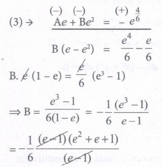
⇒ \(-\frac { 1 }{ 6 } \)(e²+e+1)
Substituting the value of A and B in (2) we get,
A-\(\frac { 1 }{ 6 } \)(e²+e+1) = -\(\frac { 1 }{ 6 } \)

⇒ A = \(\frac { 1 }{ 6 } \)(e² + e)
Substituting the value of A and B in (1) we get,
y = \(\frac { 1 }{ 6 } \)(e²+e)e^x-\(\frac { 1 }{ 6 } \)(e²+e+1)e^2x+\(\frac { { e }^{ 4x } }{ 6 } \)
⇒ 6y = (e²+e)e^x-(e²+e+1)e^2x+e^4x

Given m²\(\frac { dc }{ dm } \)+2mc = 2
Dividing by m², we get,
\(\frac { dC }{ dm } +\frac { 2c }{ m } =\frac { 2 }{ { m }^{ 2 } } \)
This is of form \(\frac { dy }{ dx } \)+Py = Q
where P = \(\frac { 2 }{ m } \) and Q = \(\frac { 2 }{ m } \)
\(\int { p } dm=\int { \frac { 2 }{ m } } \)dm = 2 log m = log m²
∴ Integrating Factor (LF.) = \(e^{ \int { P } dm }=e^{ logm^{ 2 } }\)
= m²
∴ The solution is
\(ce^{ \int { P } dm }=\int { Q } e^{ \int { P } dm }m+c.K\)
cm²=\(\int { \frac { 2 }{ { m }^{ 2 } } { m }^{ 2 } } dm+K=\int { 2 } dm+cK\)
cm² = 2m+K
Given that c = 4, when m = 2
4(2²) = 2(2) + K ⇒ 16 - 4 = K
⇒ K=12
∴ (1) becomes
cm² = 2m+ 12
⇒ cm² = 2 (m + 6)

(x² +y²) dx = -2xy dy
⇒ \(\frac { dy }{ dx } =-\frac { ({ x }^{ 2 }+{ { y }^{ 2 }) } }{ 2xy } \)
Since the numerator and denominator is a homogenous function of degree 2,
put y = vx and \(\frac { dy }{ dx } =v+x\frac { dy }{ dx } \)
x\(\frac { dv }{ dx } =-\left( \frac { { x }^{ 2 }+{ v }^{ 2 }{ x }^{ 2 } }{ 2xvx } \right) \)

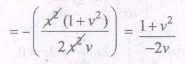
x\(\frac { dv }{ dx } =-\left( \frac { 1+{ v }^{ 2 } }{ 2v } \right) -v\)
= \(\frac { -1-{ v }^{ 2 }-2{ v }^{ 2 } }{ 2v } -\frac { -1-3{ v }^{ 2 } }{ 2v } =-\left( \frac { 1+3{ v }^{ 2 } }{ 2v } \right) \)
\(\frac { 2v.dv }{ 1+3{ v }^{ 2 } } =-\frac { dx }{ x } \)
Multiplying by 3,
put 1 + 3v² = t
6v dv = dt
\(\int { \frac { 6vdv }{ 1+3v^{ 2 } } } dv=-\int { 3 } \frac { dx }{ x } \)
\(\int { \frac { dt }{ t } } =-3\int { \frac { dx }{ x } } \)
⇒ log t = - 3 log x + log C
⇒ log (1 + 3v²) + 3 log x = log C
⇒ log (1 + 3v²) .x³ = log C
⇒ (1 + 3v²)x³= C
Replace v by \(\frac { y }{ x } \) we get,
\(\left( 1+\frac { { 3y }^{ 2 } }{ { x }^{ 2 } } \right) \).x³= C
⇒ \(\left( 1+\frac { { 3y }^{ 2 } }{ { x }^{ 2 } } \right) ^{ \frac { 1 }{ 3 } }\)= C

Given Q_d = 30 - 5p + 2\(\frac { dp }{ dt } +\frac { { d }^{ 2 }p }{ dt^{ 1 } } \) and
Q_s = -6 + 3p
At equilibrium Q_d = Q_s
⇒ 30 - 5p+2\(\frac { dp }{ dt } +\frac { { d }^{ 2 }p }{ dt^{ 1 } } \) = -6+3p
⇒ \(\frac { { d }^{ 2 }p }{ dt^{ 2 } } +2\frac { dp }{ dt } \)- 5p + 30 - 6 - p = 0
⇒ \(\frac { { d }^{ 2 }p }{ dt^{ 2 } } +2\frac { dp }{ dt } \)- 8p = 24
The auxiliary equation is m² + 2m - 8 = 0
⇒ (m + 4) (m - 2) = 0
⇒ m = - 4, 2
∴  C.F. is Ae^-4t + Be^2t
Particular Integral PI = \(\frac { -24 }{ (D+4)(D-x) } \)e0x
= \(\frac { -24 }{ (0+4)(0-2) } =\frac { -24 }{ -8 } \)=3
∴ y = CF + PI
∴ The general solution is
P = Ae^-4t + Be^2t + 3.

For market clearance, the required condition is Q_d = Q_s
⇒ \(29-2p-5\frac { dp }{ dt } +\frac { { d }^{ 2 }p }{ { dt } } =5+4p\)
⇒ \(24-6p-5\frac { dp }{ dt } +\frac { { d }^{ 2 }p }{ { dt }^{ 2 } } =0\)
⇒ \(\frac { { d }^{ 2 }p }{ { dt }^{ 2 } }+ 5\frac { dp }{ dt } -6p=-24\)
(D²−5D−6)p = –24
The auxiliary equation is
m² − 5m − 6 = 0
(m−6)(m+1) = 0
⇒ m = 6, –1
C.F = Ae^6t + Be^−t
\(P.I=\frac { 1 }{ \phi (D) } f(x)\)
= \(\frac { 1 }{ { D }^{ 2 }-5D-6 } (-24){ e }^{ 0t }\)
= \(\frac { -24 }{ -6 } \) (Replace D by 0)
= 4
The general solution is p = C.F + P.I
= Ae^6t + Be^−t + 4

(3D² + D - 14)y = 4 - 13\({ e }^{\frac{-7}{3}x}\)
The auxiliary equation is
3m² + m − 14 = 0
(3m+7)(m−2) = 0
m = \(\frac{-7}{3}\),2
C.F = \({ Ae }^{ \frac { -7 }{ 3 } x }+{ Be }^{ 2x }\)
\(=\frac { 1 }{ 3{ D }^{ 2 }+D-14 } (4)+\frac { 1 }{ { 3D }^{ 2 }+ } \left( { 4-13e }^{ \frac { -7 }{ 3 } x } \right) \)
= PI₁+ PI₂
P.I₁ = \(\frac { 1 }{ 3{ D }^{ 2 }+D-14 } 4{ e }^{ 0x }\) 
=\(\frac { 1 }{ 0+0-14 } { 4 }e^{ 0x }\)(Replace D by 0)
P.I₁ = \(\frac{-4}{14} =\frac{-2}{7} \)
P.I₂ = \(\frac { 1 }{ 3{ D }^{ 2 }+D-14 } \times { (-13)e }^{ \frac { -7 }{ 3 } x }\)
Replace D by \(\frac{-7}{3}\) Here 3D² + D − 14 = 0 when D = −\(\frac{7}{3}\)
∴ P.I₂ = x.\(\frac { 1 }{ 6D+1 } \left( -{ 13e }^{ \frac { -7 }{ 3 } x } \right) \)
Replace D by \(\frac{-7}{3}\) 
∴ P.I₂ = \(x\frac { 1 }{ 6\left( \frac { -7 }{ 3 } \right) +1 } \left( -{ 13 }e^{ \frac { -7 }{ 3 } x } \right) \)
= x\(e^{ \frac { -7 }{ 3 } x }\)
The general solution is y = C.F. + P.I₁ + P.I₂
y = \({ Ae }^{ \frac { -7 }{ 3 } x }+B{ e }^{ 2x }-\frac { 2 }{ 7 } +{ xe }^{ \frac { -7 }{ 3 } x }\)

(D² − 2D + 1)y = e^2x + e^x
The auxiliary equation is
m² − 2m + 1 = 0
⇒ (m−1)(m−1) = 0
m = 1, 1
C.F = (Ax +B)e^x
\(PI=\frac { 1 }{ \phi (D) } f(x)\) = \(\frac { 1 }{ { D }^{ 2 }-2D+1 } \)(e^2x + e^x)
P.I₁ = \(\frac { 1 }{ { D }^{ 2 }-2D+1 } \)e^2x
= \(\frac { 1 }{ 4-4+1 } \)e^2x (replace D by 2)
= e^2x
and P.I₂ = \(\frac { 1 }{ { D }^{ 2 }-2D+1 } \) e^x
= \(\frac { 1 }{ { (D-1) }^{ 2 } } { e }^{ x }\)
Replace D by 1. (D −1)² = 0 when D = 1
∴ \(P.{ I }_{ 2 }={ x }_{ 2 }.\frac { 1 }{ { 2(D-1) }^{ 2 } } { e }^{ x }\)
Replace D by 1. (D −1) = 0 when D = 1
∴ P.I₂ = x²\(\frac { 1 }{ 2 } { e }^{ x }\)
The general solution is
y = C.F + P.I₁ + P.I₂
y = (Ax +B)e^x + e^2x + \(\frac { { x }^{ 2 } }{ 2 } { e }^{ x }\)

Given Q_d = 13 - 6p + 2\(\frac { dp }{ dt } +\frac { { d }^{ 2 }p }{ dt^{ 1 } } \)  Q_s = - 3 + 2p
At equilibrium  Q_d = Q_s
⇒ 13 - 6p + 2\(\frac { dp }{ dt } +\frac { { d }^{ 2 }p }{ dt^{ 1 } } \) = - 3 + 2p
⇒ \(\frac { { d }^{ 2 }p }{ dt^{ 2 } } +2\frac { dp }{ dt } \) - 6p + 13 + 3 - 2p = 0 
⇒ \(\frac { { d }^{ 2 }p }{ dt^{ 2 } } +2\frac { dp }{ dt } \) - 8p + 16 = 0
⇒  \(\frac { { d }^{ 2 }p }{ dt^{ 2 } } +2\frac { dp }{ dt } \) - 8p = - 16
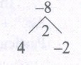
The auxiliary equation is m² + 2m - 8 = 0
⇒ (m + 4) (m - 2) = 0
⇒ m = - 4, 2
The roots are real and different.
∴ Complementary function CF is Ae^-4t + Be^2t
Particular Integral PI = \(\\ \frac { 1 }{ \phi (D) } \).f(t)
=\(\frac { 1 }{ { D }^{ 2 }+2D-8 } .(-16)=\frac { -16.e^{ 0x } }{ (D+4)(D-2) } \)
PI = \(\frac { -16 }{ (0+4)(0-2) } =\frac { -16 }{ -8 } \) = 2
∴ P = CF + PI
∴ The general solution is
P = Ae^-4t + Be^2t + 2

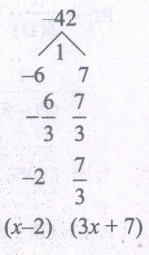
The auxiliary equation is 3m² + m -14 = 0
(m-2)\(\frac { 7 }{ 3 } \) = 0
⇒ m = 2, -\(\frac { 7 }{ 3 } \)
The roots are real and different
∴ CF is Ae^2x+\(Be^{ -\frac { 7 }{ 3 } x }\)
Particular Integral PI = \(\frac { 1 }{ \phi (D) } \).f(x)
PI = \(\frac { 1 }{ (3D^{ 2 }+D-14) } \).13 e2x
= \(\frac { 13.e^{ 2x } }{ 3D^{ 2 }+D-14 } \)
= \(\frac { 13e^{ 2x } }{ (D-2)(3D+7) } =\frac { 13e^{ 2x } }{ 3(D-2)\left( D+\frac { 7 }{ 3 } \right) } \)
= \(\frac { 13x{ e }^{ 2x } }{ 3\left( 2+\frac { 7 }{ 3 } \right) } \)

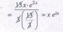
∴ y = CF + PI
∴ The general solution is
y = Ae^2x+\({ Be }^{ -\frac { 7 }{ 3 } x }\) + xe^2x

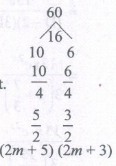
The auxiliary equation is 4m² + 16m + 15 = 0
(2m +5) (2m +3) = 0
⇒ m = \(-\frac { 3 }{ 2 } ,\frac { 5 }{ 2 } \)
The roots are real and different.
∴ Complementary function
CF is \(A{ e }^{ -\frac { 3 }{ 2 } x }+Be^{ -\frac { 5 }{ 2 } x }\)
Particular Integral PI = \(\frac { 1 }{ \phi D } \).f(x)
PI = \(\frac { 1 }{ (2D+5)(2D+3) } .4.e^{ -\frac { 3 }{ 2 } x }\)

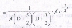
= \(\frac { xe^{ -\frac { 3 }{ 2 } x } }{ \left( -\frac { 3 }{ 2 } +\frac { 5 }{ 2 } \right) } \) [∵ D + \(\frac { 3 }{ 2 } \) = 0 when D = -\(\frac { 3 }{ 2 } \)]
= \(\frac { x.e^{ -\frac { 3 }{ 2 } x } }{ 1 } =x.e^{ -\frac { 2 }{ 2 } x }\)
∴ y = CF + PI₁ + PI₂
∴ The general solution is
y =\(Ae^{ -\frac { 3 }{ 2 } x }+Be^{ -\frac { 5x }{ 2 } }+xe^{ -\frac { 3 }{ 2 } x }\).

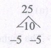
The auxiliary equation is m² - 10m + 25 = 0
(m - 5) = 0
⇒ m = 5, 5
The roots are real and equal.
∴ Complementary function CF is (Ax + B) e_5x
Particular Integral PI1 =\(\frac { 1 }{ \phi (D) } \)f₁(x)
= \(\frac { 1 }{ (D-5)^{ 2 } } \).4 x e^5x = 4.e^5x.\(\frac { x^{ 2 } }{ 2 } \)
= 2x² e^5x [∵ (D-5)² =0 when D=5]
PI₂ = \(\frac { 1 }{ \phi (D) } \)f₂(x)
= \(\frac { 1 }{ (D-5)^{ 2 } } 5=\frac { 5.{ e }^{ 0x } }{ (D-5)^{ 2 } } =\frac { 5.{ e }^{ 0x } }{ (0-5)^{ 2 } } \)
= \(\frac { 5 }{ 25 } =\frac { 1 }{ 5 } \)
∴ y = CF + PI₁ + PI₂
∴ The general solution is
y = (Ax + B) e^5x + 2x² e^5x + 5

The auxiliary equation is m² + m - 6 = 0
⇒ (m + 3) (m - 2) = 0
⇒ m = -3, 2
The roots are real and different.
∴ The complementary function CF is Ae^-3x + B^ex
Particular Integral
PI₁=\(\frac { 1 }{ \phi (D) } \)f₁(x)
=\(\frac { 1 }{ ({ D }^{ 2 }+D-6) } \)e^3x
PI₁=\(\frac { { e }^{ 3x } }{ (D+3)(D-2) } =\frac { { e }^{ 3x } }{ (3+3)(3-2) } \)
= \(\frac { { e }^{ 3x } }{ 6(1) } =\frac { e^{ 3x } }{ 6 } \)
PI₂ = \(\frac { 1 }{ \phi (D0 } { f }_{ 2 }(x)=\frac { e^{ -3x } }{ (D+3)(D-2) } \)
= x\(\frac { { e }^{ -3x } }{ (-3-2) } \) [∵ when D = - 3, D + 3 = 0]
PI₂ = \(-\frac { x }{ 5 } \)e^-3x
∴ y = CF+PI₁+PI₂
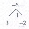
∴ The general solution is
y = Ae^-3x+Be^2x+\(\frac { { e }^{ 3x } }{ 6 } -\frac { x }{ 5 } \)e^-3x

Auxiliary equation is m² - 3m + 2 = 0
∴ (m - 1)(m - 2) = 0
⇒ m = 1,2
∴ Complementary function CF is A^ex + Be^2x
PI = \(\frac { 1 }{ \phi (D) } \)(x)
= \(\frac { 1 }{ { D }^{ 2 }-3D+2 } \).e3x
= \(\frac { 1 }{ (D-1)(D-2) } \).e3x
= \(\frac { e^{ 3x } }{ (3-1)(3-2) } \).e3x
= \(\frac { { e }^{ 3x } }{ 2 } \)
General solution is y = CF + PI
y = A^ex+Be^2x+\(\frac { 1 }{ 2 } \)e^3x ...(1)
Given when x = 0, y = 0
∴ 0 = Ae⁰+Be₀+\(\frac { 1 }{ 2 } \)e₀ ⇒ 0 = A+B-\(\frac { 1 }{ 2 } \) ..(2)
Also, when x = log2, y = 0
⇒ 0 = Ae^log2+Be^2log2+e^3log3
⇒ 0 = A(2)+\(Be^{ log2^{ 2 }+ }+\frac { 1 }{ 2 } elog2^{ 3 }\)
⇒ 0 = 2A+4B+\(\frac{8}{2}\) ⇒ 2A+4B=-4
⇒ A+2B = -2
(2)-(3) ⇒ A+B = -\(\frac { 1 }{ 2 } \)

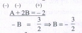
Substituting B = -\(\frac { 3 }{ 2 } \) in  (2) we get
\(A-\frac { 3 }{ 2 } =-\frac { 1 }{ 2 } \Rightarrow A=-\frac { 1 }{ 2 } +\frac { 3 }{ 2 } \Rightarrow \frac { 2 }{ 2 } \)=1
∴ y = \(1.e^{ x }-\frac { 3 }{ 2 } e^{ 2x }+\frac { e^{ 3x } }{ 2 } \).

Let p(t) denotes the amount of moiley in the account at time t.
Then the differential equation governing the growth of money is
\(\frac { dp }{ dt } =\frac { 8p }{ 100 } \)
⇒ \(\frac { dp }{ dt } \) = .08p
⇒ \(\frac { dp }{ p } \)= .08dt
Integrating both sides we get,
\(\int { \frac { dp }{ p } = } \int { -08 } dt\)
⇒ logp= .08t+c
⇒ P = e^.08t e^c
⇒ p = c₁e^.08t where c₁ = e^x
when t = 0, p = Rs.1,00,000
∴ (1) becomes 1,00,000 = c₁e^.08(0)
⇒ 1,00,000 = c₁
∴ (1) p = 1,00,000 e^0.08t
when t = 10,
p =1,00,000 e^0.08(10)
= 1,00,000 (e^0.8)
= 1,00,000(2.2255)
[∵ e^0.8 = 2.225540]
Rs. 2,22,554

The given differential equation is of the form
\(\frac { dy }{ dx } \)+ Py = Q where
P =\(\frac { 1 }{ x } \); Q = xe^x
∴ \(\int { p } dx=\int { \frac { 1 }{ x } } \) = logx
∴ Integratin'cg tactor (I. F) = \(e^{ \int { p } dx }=e^{ logx }=x\)
Hence the solution is
\(ye^{ \int { p } dx }=\int { Q } .e^{ \int { p } dx }dx+c\)
⇒ yx =\(\int { x{ e }^{ x }dx+c } \)
⇒ xy = \(\int { x{ e }^{ x }dx+c } \) ....(1)
Let u = x²; dv = e^x
u' = 2x; v = e^x
u" = 2; v₁ = e^x
v₂ = e^x
Using Bernoulli's formula,
\(\int { u } dv\) = uv - u'v₁+ u"v₂
∴ (1) becomes
xy = x²e^x - 2xe^x + 2e^x+c
⇒ xy = e^x(x²-2x+2) + c

Given differential equation is of the form
\(\frac { dy }{ dx } \)+Py = Q where
P = 2 tanx; Q = sinx
\(\int { p } dx=\int { 2 } \tan xdx\) = 2(log secx) = log sec²x
∴ Integrating factor (I. F) =\(e^{ \int { p } dx }=e^{ log\quad sec^{ 2x } }\)
= sec²x
Hence the solution is
\(ye^{ \int { p } dx }=\int { Q } .e^{ \int { p } dx }dx+c\)
⇒ y sec²x =\(\int { \sin x }\ { \sec }^{ 2 }x\ dx\)+c
⇒ y sec²x =\(\int { \sin x } .\frac { 1 }{ \cos^{ 2 }x } \) dx + c
⇒ y sec²x =\(\int { \frac { \sin x }{ \cos x } .\frac { 1 }{ \cos x } } \) dx + c
⇒ y sec²x =\(\int { \tan x } \) sec x dx + c
⇒ y sec²x = sec x + c ...(1)
Also its given when x = \(\frac { \pi }{ 3 } \), y = 0
∴ 0\(({ sec }^{ 2 }\frac { \pi }{ 3 } )=sec\frac { \pi }{ 3 } +c\)
⇒ 0 = 2+c ⇒ c = -2
∴ (1) becomes
y sec 2x = sec x-2

The given differential equation is of this form
\(\frac { dy }{ dx } \)+Py=Q where
P = tan x; Q = cos³x
∴ \(\int { p } dx=\int { \tan x } dx\) = log secx
∴ Integrating factor (I.F) = \(e^{ \int { p } dx }\) = e^{logx secx}
= sec x
Hence, the solution is
\(ye^{ \int { p } dx }=\int { Q } .e^{ \int { p } dx }dx+c\)
⇒ y sec x =\(\\ \int { cos^{ 3 }x } \)dx+c
[∴ cos 2x = 2cos²x-1]
⇒ 2 cos²x = 1 + cos2x
⇒ cos²x = \(\frac { 1+cos2x }{ 2 } \)]
⇒ y secx = \(\int { \cos^{ 3 }x.\frac { 1 }{ \cos x } } \)dx+c
⇒y sec x =\(\int { cos^{ 2 }x } dx+c\)
⇒ y sec x =\(\int { \left( \frac { 1+cos2x }{ 2 } \right) } dx+c\)
⇒ y sec x = \(\frac { 1 }{ 2 } \left[ x+\frac { \sin 2x }{ 2 } \right] \)+c

The given differential equation is of the form
\(\frac { dy }{ dx } \)+ Py = Q where
P = \(\frac { 1 }{ x } \); Q = xe^x
∴ \(\int { p } dx=\int { \frac { 1 }{ x } } \) = log x
∴ Integrating factor (I. F) = \(e^{ \int { p } dx }=e^{ logx }=x\)
Hence the solution is
\(ye^{ \int { p } dx }=\int { Q } .e^{ \int { p } dx }dx+c\)
⇒ yx = \(\int { x{ e }^{ x }dx+c } \)
⇒ xy =\(\int { x{ e }^{ x }dx+c } \)....(1)
Let u = x²; dv = e^x
u' = 2x; v = e^x
u" = 2; v₁ = e^x
v₂ = e^x
Using Bernoulli's formula,
\(\int { u } dv\) = uv-u'v₁+u"v₂
∴ (1) becomes
xy = x²e^x - 2xe^x + 2e^x+c
⇒ xy = e^x(x²-2x+2) + c

The given differential equation is of this form
\(\frac { dy }{ dx } \)+Py = Q Where
P = \(\frac { 3x^{ 2 } }{ 1+{ x }^{ 3 } } \); Q=\(\frac { 1+x^{ 2 } }{ 1+{ x }^{ 3 } } \)
∴ \(\int { p } dx=\int { \frac { 3x^{ 2 } }{ 1+{ x }^{ 3 } } } \)dx
put t = 1+x³ ⇒ dt = 3x² dx
=\(\int { \frac { dt }{ t } } \) = log t =log(1+x³) [∵ t = 1+x³]
∴ Integrating factor (I. F) = \(e^{ \int { p } dx }=e^{ log(1+x^{ 3 }) }\)
= 1 + x³
Hence the solution is
\(ye^{ \int { p } dx }=\int { Q } .e^{ \int { p } dx }dx+c\)

=\(\int { (1+{ x }^{ 2 }) } dx\) + c
⇒ y(1+x³) = x + \(\frac { { x }^{ 3 } }{ 3 } \) + c

\(\frac { dy }{ dx } +\frac { 2 }{ y } y\) = x³
The given differential equation is of this form [Divided by x]
\(\frac { dy }{ dx } \)+Py = Q where
P =\(\int { \frac { 2 }{ x } } \) and Q = x³
∴ \(\int { P } dx=\int { \frac { 2 }{ x } dx } \) = 2 log x = log x²
∴ Integrating factor (I. F) =\(e^{ \int { p } dx }=e^{ logx^{ 2 } }\)= x²
Hence the solution is
\(ye^{ \int { p } dx }=\int { Q } .e^{ \int { p.dx } }dx+c\)
⇒ y.x² = \(\int { { x }^{ 3 }.{ x }^{ 2 } } dx+c\)
⇒ x²y =\(\\ \int { { x }^{ 5 }dx } +c\)
⇒ x²y = \(\frac { { x }^{ 6 } }{ 6 } \) + c

\(x\frac { dC }{ dx } =\frac { 3 }{ x } -C\)
\(x\frac { dC }{ dx } =\frac { 3 }{ x^2 } -\frac {C}{x}\)
\(\frac { dC }{ dx } +\frac { C }{ x } =\frac { 3 }{ { x }^{ 2 } } \)
i.e., \(\frac { dC }{ dx } +\frac { C }{ x } =\frac { 3 }{ { x }^{ 2 } } \)
It is of the form \(\frac { dC }{ dx } +PC=Q\)
Here, \(P=\frac { 1 }{ x } ,Q=\frac { 3 }{ { x }^{ 2 } } \)
ഽPdx = ഽ\(\frac 1 x\)dx = log x
I.F = eഽ^pdx = e^{log x} = x
The Solution is
C(I.F) = ഽQ(I.F)dx + k where k is constant
Cx = ഽ\(\frac{3}{x^2}\)xdx + k
= 3ഽ\(\frac 1 x\) dx + k
Cx = 3log x + k  (1)
Given C = 2 When x = 1
(1) ⇒ 2 × 1 ⇒ k =2
∴ The relationship between C and x is
Cx = 3 log x + 2

Given \(\frac { dy }{ dx } \) − (3 cot x) y = sin 2x
It is of the form \(\frac { dy }{ dx } \) + Py = Q
Here P= − 3 cot x,Q = sin 2x
ഽPdx = ഽ-3 cot xdx = -3 log sin x = - log sin³x = log \(\frac { 1 }{ { sin }^{ 3 }x } \)
I.F. = \({ e }^{ log\frac { 1 }{ { sin }^{ 3 }x } }=\frac { 1 }{ { sin }^{ 3 }x } \)
The required solution is y (I.F) = ഽQ(I.F)dx+c
\(y\frac { 1 }{ { sin }^{ 3 }x } =\int { sin2x } \frac { 1 }{ { sin }^{ 3 }x } dx+c\)
\(\int { \frac { 1 }{ { sin }^{ 3 }x } } =\int { 2sinxcosx\times \frac { 1 }{ { sin }^{ 3 }x } } dx+c\)
= \(2\int { \frac { 1 }{ sinx } \times \frac { cosx }{ sinx } } dx+c\)
= ഽcos ecx cot xdx + c
\(y\frac { 1 }{ { sin }^{ 3 }x } =-2cosecx+c\)
Now y = 2 when x = \(\frac { \pi }{ 2 } \)
(1) ⇒ 2\(\frac {1 }{ 1 } \) = −2×1+c ⇒ c= 4
∴ (1) ⇒ \(y\frac { 1 }{ { sin }^{ 3 }x } \) = −2cosecx + 4

The given equation can be reduced to
\(\frac { dy }{ dx } +\frac { 2x }{ { x }^{ 2 }+1 } y=\frac { 4{ x }^{ 2 } }{ { x }^{ 2 }+1 } \)
It is of the form \(\frac { dy }{ dx } \) + Py = Q
Here P \(=\frac { 2x }{ { x }^{ 2 }+1 } ,Q=\frac { 4{ x }^{ 2 } }{ { x }^{ 2 }+1 } \)
ഽPdx = ഽ\(\frac { 2x }{ { x }^{ 2 }+1 } \)dx = log(x² +1)
I.F = e^ഽpdx = e^log(x2+1) = x² + 1
The required solution is y(IF) = ഽQ(I.F)dx + c
y(x² +1) = ഽ\(\frac { 4{ x }^{ 2 } }{ { x }^{ 2 }+1 } \)(x² + 1)dx + c
y(x² +1) = \(\frac { 4{ x }^{ 3 } }{ 3 } \) + c

The given equation can be written as \(\frac { dy }{ dx } +\frac { 1 }{ { cos }^{ 2 }x } y=\frac { tanx }{ { cos }^{ 2 }x } \)
\(\frac { dy }{ dx } \) + y sec²x = tan x sec²x
It is of the form \(\frac{dy}{dx}\) + Py + Q
Here P = sec²x,Q = tanx sec²x
ഽPdx = ഽsec² x dx = tanx
I.F = eഽ^pdx = e^{tan x}
The required solution is y(I.F) = ഽQ(I.F)dx + c
ye^{tan x} = ഽtan x sec²xe^tan xdx + c
Put tan x = t
Then sec² xdx = dt
∴ ye^{tan x} = ഽte^t dt + c
= ഽtd(e^t) + c
= te^t − e^t + c
= tanx e^{tan x}−e^{tan x}+ c
ye^{tan x} = e^{tan x}(tan x − 1) + c

(x² + y²)dy = xydx 
⇒ \(\frac { dy }{ dx } +\frac { xy }{ x^{ 2 }+{ y }^{ 2 } } \)....(1)
Since the numerator and denominators are homogeneous functions of degree 2,
put y = vx, and \(\frac { dy }{ dx } =v+x\frac { dv }{ dx } \)
(1) becomes

= \(\frac { v }{ 1+v^{ 2 } } \)
⇒ v+\(x\frac { dv }{ dx } =\frac { v }{ 1+v^{ 2 } } -v=\frac { v-v(1+v^{ 2 }) }{ 1+{ v }^{ 2 } } \)
= \(\frac { v-v-{ v }^{ 3 } }{ 1+v } \)
= \(\frac { -v^{ 3 } }{ 1+v^{ 2 } } \)
Separating the variables we get,
\(x\frac { dv }{ dx } =\frac { -v^{ 3 } }{ 1+v^{ 2 } } \)
⇒ \(\frac { (1+v^{ 2 })dv }{ { v }^{ 3 } } =\frac { -dx }{ x } \)
⇒ \(\frac { 1 }{ { v }^{ 3 } } dv+\frac { { v }^{ 2 } }{ { v }^{ 3 } } dv=-\int { \frac { dx }{ x } } \)
⇒ \(\frac { 1 }{ { v }^{ 3 } } dv+\frac { dv }{ v } =-\frac { dx }{ x } \)
Integrating both sides we get,
\(\int { v^{ -3 }dv } +\int { \frac { dv }{ v } } =-\int { \frac { dx }{ x } } \)
\(\frac { -1 }{ 2v^{ 2 } } \) + log v = -log x + log c
⇒ \(\frac { 1 }{ 2v^{ 2 } } \) = log v + log x - log c
⇒ \(\frac { 1 }{ 2v^{ 2 } } =log\frac { vx }{ c } \)
Replace v by \(\frac { y }{ x } \) we get,

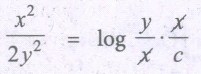
⇒ \(\frac { { x }^{ 2 } }{ 2{ y }^{ 2 } } =log\frac { y }{ c } \)
⇒ \(e^{ { x }^{ 2 }/2{ y }^{ 2 } }=\frac { y }{ c } \)
⇒ y = \(ce^{ { x }^{ 2 }/2{ y }^{ 2 } }\).

Given (y³−2yx²)dx + (2xy²−x³)dy = 0
(y³−2yx²)dx = - (2xy²−x³)dy
(y³−2yx²)dx = - (x³-2xy²)dy
⇒ \(\frac { dy }{ dx } =\frac { { y }^{ 3 }-2yx^{ 2 } }{ { x }^{ 3 }-2xy^{ 2 } } \)
Since the numerator and denominator are homogeneous functions of degree 3,
put y = vx and \(\frac { dy }{ dx } =v+x\frac { dv }{ dx } \)

⇒ \(v+x\frac { dv }{ dx } =\frac { { v }^{ 3 }-2v }{ 1-2v^{ 2 } } \)
⇒ \(x\frac { dv }{ dx } =\frac { { v }^{ 3 }-2v }{ 1-2v^{ 2 } } -v=\frac { { v }^{ 3 }-2v-v(1-2v^{ 2 }) }{ 1-2v^{ 2 } } \)
⇒ \(x\frac { dv }{ dx } =\frac { { v }^{ 3 }-2v-v+2v^{ 3 } }{ 1-2v^{ 2 } } =\frac { { v }^{ 3 }+2v^{ 3 }-3v }{ 1-2v^{ 2 } } \)
= \(\frac { 3v^{ 3 }-3v }{ 1-2v^{ 2 } } \)
Separating the variables we get,
\(\frac { 1-2v^{ 2 } }{ 3v^{ 3- }3v } dv=\frac { dx }{ x } \)
⇒ \(\frac { 1-2v^{ 2 } }{ { v }^{ 3 }-v } dv=3\frac { dx }{ x } \)
\(\frac { 1-2v^{ 2 } }{ { v }^{ 3 }-v } =\frac { 1-2v^{ 2 } }{ v({ v }^{ 3 }-1) } \)
= \(\frac { 1-2v^{ 2 } }{ v(v+1)(v-1) } \)
= \(\frac { A }{ v } +\frac { B }{ v+1 } +\frac { C }{ v-1 } \)
1-2v² = A(v+1)(v-1)+Bv(v-1)+Cv(v+1)
put v = 1 ⇒ -1 = 2c ⇒ c = -\(\frac { 1 }{ 2 } \)
put v = -1 ⇒ -1 = -B = -\(\frac { 1 }{ 2 } \)
put v = -1 ⇒ -1 = -B(-2)
⇒ -1 = 2B ⇒ B = -\(\frac { 1 }{ 2 } \)
put v = 0 ⇒ 1 = -A + 0 + 0
⇒ A = -1
⇒ \(\int { \left( \frac { -1 }{ v } \frac { -\frac { 1 }{ 2 } }{ v+1 } \frac { -\frac { 1 }{ 2 } }{ v-1 } \right) } dv=3\int { \frac { dx }{ x } } \)
⇒ -log v -\(\frac { 1 }{ 2 } \)log(v+1) -\(\frac { 1 }{ 2 } \)log(v-1)
= 3log x + log c
⇒ -\(\frac { 1 }{ 2 } \)log(v-1) = 3log x + log c
⇒ log v+\(\frac { 1 }{ 2 } \)log(v+1)+\(\frac { 1 }{ 2 } \)log(v-1)
= -3log x + log c
⇒ log v.\(\sqrt { v+1 } \sqrt { v-1 } =log\left( \frac { 1 }{ x^{ 3 } } \right) \).c
⇒ v\(\sqrt { v^{ 2 }-1 } =\frac { c }{ { x }^{ 3 } } \)
Replace v by \(\frac { y }{ x } \) we get,
\(\frac { y }{ x } \sqrt { \frac { { y }^{ 2 } }{ x^{ 2 } } -1 } =\frac { c }{ { x }^{ 3 } } \)
⇒ \(\frac { y }{ x } \sqrt { \frac { { y }^{ 2 }-{ x }^{ 2 } }{ x } } =\frac { c }{ { x }^{ 3 } } \)
⇒ \(\sqrt { { y }^{ 2 }-x^{ 2 } } =\frac { c }{ x } \Rightarrow \sqrt { { y }^{ 2 }-x^{ 2 } } \)= c        (1)
Since the curve passes through (1, 2) we get
(1) (2) \(\sqrt { 4-1 } =c\Rightarrow c=2\sqrt { 3 } \)
Substituting c = \(2\sqrt { 3 } \) in (1) we get
\(xy\sqrt { { y }^{ 2 }-x^{ 2 } } =2\sqrt { 3 } \).

(y² − 2xy)dx = (x² − 2xy)dy
⇒ \(\frac { dy }{ dx } =\frac { { y }^{ 2 }-2xy }{ { x }^{ 2 }-2xy } \)
Since the numerator and denominator are homogeneous functions of degree 2,
put y = vx and \(\frac { dy }{ dx } =v+x\frac { dv }{ dx } \)

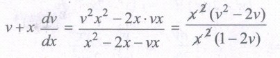
=\(\frac { { v }^{ 2 }-2v }{ 1-2v } \)
⇒ \(x\frac { dv }{ dx } =\frac { { v }^{ 2 }-2v }{ 1-2v } -v=\frac { { v }^{ 2 }-2v-v(1-2v) }{ 1-2v } \)
=\(\frac { { v }^{ 2 }-2v-v+2v^{ 2 } }{ 1-2v } \)
⇒ \(x\frac { dv }{ dx } =\frac { 3v^{ 2 }-3v }{ 1-2v } \)
Separating the variables we get,
\(\frac { (1-2v)dv }{ 3v^{ 2 }-3v } =\frac { dx }{ x } \)
= \(-\frac { (2v-1)dv }{ { v }^{ 2 }-v } =3\frac { dx }{ x } \)
Integrating both sides we get,
\(-\int { \frac { (2v-1)dv }{ { v }^{ 2 }-v } } =3\int { \frac { dx }{ x } } \)
⇒ -log(v²-v) = 3logx + log c
⇒ log x³ + log(v²-v) = -log c = log k
[where log k = -log c]
⇒ log x³(v²-v) = log k
⇒ x³(v²-v) = k
Repalce v by \(\frac { y }{ x } \) we get,
\({ x }^{ 3 }\left( \frac { { y }^{ 2 } }{ { x }^{ 2 } } -\frac { y }{ x } \right) \)= k
⇒ \({ x }^{ 3 }\left( \frac { { y }^{ 2 }-xy }{ { x }^{ 2 } } \right) \)= k
⇒ x(y²-xy) = k

Since the numerator and denominator homogeneous function of degree 1,
put y = vx and  \(\frac { dy }{ dx } =v+x\frac { dv }{ dx } \)

\(x\frac { dv }{ dx } =\frac { (3-2v) }{ (2-3v) } -v=\frac { 3-2v-v(2-3v) }{ 2-3v } \)
\(x\frac { dv }{ dx } =\frac { 3-2v-2v-3v^{ 2 } }{ 2-3v } =\frac { 3-4v-3v^{ 2 } }{ 2-3v } \)
Separating the variables we get,
\(\frac { (2-3v)dv }{ 3{ v }^{ 2 }-4v+3 } =\frac { dx }{ x } \)
Integrating both sides we get,
⇒ \(\int { \frac { (2-3v)dv }{ 3{ v }^{ 2 }-4v+3 } } =\int { \frac { dx }{ x } } \)
Multiplying by -2 both sides we get,
⇒ \(\int { \frac { -2(2-3v)dv }{ 3v^{ 2 }-4v+3 } } =-2\int { \frac { dx }{ x } } \)
⇒ \(\int { \frac { (6v-4)dv }{ 3v^{ 2 }-4v+3 } } =-2\int { \frac { dx }{ x } } \)
Put t = 3v² -4v+3 ⇒ dt = (6v-4)dt
⇒ \(\int { \frac { dt }{ t } } =\int { \frac { dx }{ x } } \) 
⇒ log t = -2 log x + log c
⇒ log t + log x² = log c
⇒ log tx² = logc
⇒ (3v²-4v+3)x² = c
Repalcing v by \(\frac{y}{x}\) we get,
\(\left( \frac { 3y^{ 2 } }{ x^{ 2 } } -\frac { 4y }{ x } +3 \right) x^{ 2 }\)= c
⇒ \(\left( \frac { 3{ y }^{ 2 }-4xy+3x^{ 2 } }{ { x }^{ 2 } } \right) .{ x }^{ 2 }\)= c
⇒ 3y²-4xy+x²= c

\(x\frac { dy }{ dx } =y+\sqrt { { x }^{ 2 }+{ y }^{ 2 } } \)
\(\frac { dy }{ dx } =\frac { \left[ y+\sqrt { { x }^{ 2 }+{ y }^{ 2 } } \right] }{ x } \)
Since the numerator and denominator is a homogeneous function of degree 1,
put y = vx and \(\frac { dy }{ dx } =v+x\frac { dv }{ dx } \)
∴ v + x\(\frac { dv }{ dx } =\frac { vx+\sqrt { { x }^{ 2 }+{ v }^{ 2 }{ x }^{ 2 } } }{ x } =\frac { vx+x\sqrt { 1+{ v }^{ 2 } } }{ x } \)

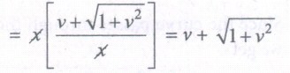
⇒ x\(\frac { dv }{ dx } =v+\sqrt { 1+{ v }^{ 2 } } -v=\sqrt { 1+v^{ 2 } } \)
Separating the variables we get,
\(\frac { dx }{ \sqrt { 1+{ v }^{ 2 } } } =\frac { dx }{ x } \)
Integrating both sides we get,
\(\int { \frac { dv }{ \sqrt { 1+{ v }^{ 2 } } } } =\int { \frac { dx }{ x } } \)
\(\left[ \therefore \int { \frac { dx }{ \sqrt { { x }^{ 2 }+a^{ 2 } } } } =log\left| x+\sqrt { { x }^{ 2 }+{ a }^{ 2 } } +c \right| \right] \)
⇒ \(log\left| v+\sqrt { { v }^{ 2 }+1 } \right| \) =log x + log c
⇒ \(log(v+\sqrt { { v }^{ 2 }+1 } )\) =log xc
⇒ v+\(\sqrt { { v }^{ 2 }+1 } \)= xc
Replace v by \(\frac { y }{ x } \) we get,
\(\frac { y }{ x } +\sqrt { \frac { { y }^{ 2 } }{ { x }^{ 2 } } +1 } \)= xc
⇒ \(\frac { y }{ x } +\sqrt { \frac { { x }^{ 2 }+{ y }^{ 2 } }{ x } } \)= xc
⇒ y+\(\\ \frac { y+\sqrt { \frac { { x }^{ 2 }+{ y }^{ 2 } }{ x } } }{ x } \)= xc
⇒ y+\(\sqrt { { x }^{ 2 }+{ y }^{ 2 } } \) = x²c

\(\frac { dy }{ dx } =\frac { x+3y }{ x-y } \)
Since the numerator and denominator are homogeneous functions of degree 1,
put y = vx and \(\frac { dy }{ dx } \) = v + x\(\frac { dv}{ dx } \)

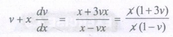
⇒ x\(\frac { dv }{ dx } =\frac { 1+3v }{ 1-v } -v=\frac { 1+3v-v(1-v) }{ 1-v } \)
= \(\frac { 1+3v-v+v^{ 2 } }{ 1-v } \)
⇒ \(x\frac { dv }{ dx } =\frac { 1+2v+v^{ 2 } }{ 1-v } \)
separating the variables we get,
\(\frac { 1-v }{ 1+2v+{ v }^{ 2 } } dv=\frac { dx }{ x } \)
⇒ \(\int { \frac { (1-v)dv }{ { v }^{ 2 }+2v+1 } } =\int { \frac { dx }{ x } } \)
⇒ \(\int { \frac { (1-v)dv }{ (v+1)^{ 2 } } } \) = log x + log c
\(\frac { 1-v }{ (v+1)^{ 2 } } =\frac { A }{ v+1 } +\frac { B }{ (v+1)^{ 2 } } \)
1-v = A(v+1)+B
put v = -1,
2 = B
1 = A + B ⇒ 1 = A+2
⇒ A = -1
∴ \(\frac { 1-v }{ (v+1)^{ 2 } } =\frac { -1 }{ v+1 } +\frac { 2 }{ (v+1) } \)
⇒ \(\int { \frac { -1 }{ v+1 } } dv+\int { \frac { 2 }{ (v+1)^{ 2 } } } dv\) = log xc
⇒ -log (v+1) - \(\frac { 2 }{ v+1 } \) = log xc
⇒ \(\frac { -2 }{ v+1 } \) = log xc + log(v+1)
⇒ \(\frac { -2 }{ v+1 } \) = log xc(v+1)
Replace v by \(\frac{y}{x}\) we get,
\(\frac { -2 }{ \frac { y }{ x } +1 } =logxc\left( \frac { y }{ x } +1 \right) \)

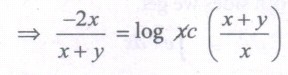
⇒ \(\frac { -2x }{ x+y } \) = logc (x+y)
⇒ e^-2x/x+y  = c(x+y)
⇒ x+y = \(\frac { 1 }{ c } \) e^-2x/x+y
⇒ x+y = ke^-2x+x+y where k = \(\frac { 1 }{ c } \).

\(\frac { dy }{ dx } =\frac { x+y }{ x } \)
Since the numerator and denominator are homogeneous functions of degree 1,
put y = vx ⇒ \(\frac { dy }{ dx } =v(1)+x.\frac { dv }{ dx } \)
∴ v + x\(\frac { dv }{ dx } \) = \(\frac { x+vx }{ x } \)

⇒ x\(\frac { dv }{ dx } \) = 1 + v - v = 1
⇒ x\(\frac { dv }{ dx } \) = 1
Separating the variables we get
\(\frac { dv }{ 1 } =\frac { dx }{ x } \)
Integrating both sides we get,
\(\int { dv } =\int { \frac { dx }{ x } } \)
\(\int { \frac { dx }{ x } } =\int { dv } \) ⇒ log x = v + log c
⇒ log\(\left( \frac { x }{ c } \right) =v\Rightarrow \frac { x }{ c } \) = e^v
x = c.ev
Replace v by y/x we get,
x = ce^y/x.

Given that \(MR=\frac { dy }{ dq } =\frac { { q }^{ 2 }+{ 3 }y^{ 2 } }{ 2qy } \)  (1)
Put y = vq and \(\frac { dy }{ dq } =v+q\frac { dv }{ dq } \) in (1)
Now (1) becomes
\(v+q\frac { dy }{ dq } =\frac { { q }^{ 2 }+{ 3 }v^{ 2 }{ q }^{ 2 } }{ 2yvq } \)
\(=\frac { 1+3{ v }^{ 2 } }{ 2v } \)
\(q\frac { dv }{ dq } =\frac { 1+3{ v }^{ 2 } }{ 2v } -v\)
\(=\frac { 1+3{ v }^{ 2 }-2{ v }^{ 2 } }{ 2v } \)
\(=\frac { { 1+v }^{ 2 } }{ 2v } \)
\(\frac { 2v }{ { 1+v }^{ 2 } } dv=\frac { dq }{ q } \)
On Integration
\(ഽ\frac { 2v }{ { 1+v }^{ 2 } } dv=ഽ\frac { dq }{ q } \)
log (1+ v²) = log q + log c
1+ v² = cq
Replace \(v=\frac { y }{ q } \)
\(1+\frac { { y }^{ 2 } }{ { q }^{ 2 } } \) = cq
q² + y² = c q³ (2)
Given output is 1 unit and revenue is Rs. 5
∴ (2) ⇒ 1 + 25 = c ⇒ c = 26
∴ The total revenue function is q² + y² = 26q³

Given marginal cost function is (x² + xy)dy + (3xy + y²)dx = 0 
\(\frac { dy }{ dx } =\frac { -(3xy+{ y }^{ 2 }) }{ { x }^{ 2 }+xy } \)    (1)
Put y = vx and \(\frac { dy }{ dx } =v+x\frac { dv }{ dx } \) in (1)
\(v+x\frac { dv }{ dx } =\frac { -(3xvx+{ v }^{ 2 }{ x }^{ 2 }) }{ { x }^{ 2 }+xvx } \)
\(=\frac { -(3v+{ v }^{ 2 }) }{ 1+v } \)
Now, \(x\frac { dv }{ dx } =\frac { -3v-{ v }^{ 2 } }{ 1+v } -v\)
\(=\frac { -3v-{ v }^{ 2 }-v-{ v }^{ 2 } }{ 1+v } \)
\(x\frac { dv }{ dx } =\frac { -4v-{ 2v }^{ 2 } }{ 1+v } \)
\(\frac { 1+v }{ 4v+2{ v }^{ 2 } } dv=\frac { -dx }{ x } \)
On Integration
\(\int { \frac { 1+v }{ 4v+2{ v }^{ 2 } } } =-\int { \frac { dx }{ x } } \)
Now, multiply 4 on both sides
\(\int { \frac { 1+v }{ 4v+2{ v }^{ 2 } } } =-4\int { \frac { dx }{ x } } \)
log (4v+2v²) = −4 logx+logc
4v + 2v² = \(\frac { c }{ { x }^{ 4 } } \)
x⁴(4v + 2v²) = c
Replace \(v=\frac { y }{ x } \)
\({ x }^{ 4 }\left( 4\frac { y }{ x } +2\frac { { y }^{ 2 } }{ { x }^{ 2 } } \right) =c\)
\({ x }^{ 4 }\left[ \frac { 4xy+2{ y }^{ 2 } }{ { x }^{ 2 } } \right] \) = c
c = 2x²(2xy + y²)   (2)
Cost of producing a pair of shoes = Rs. 12
(i.e) y = 12 when x = 2
c = 8[48 + 144]= 1536
∴ The cost function is x²(2xy + y²) = 768

x²dy + y(x + y) dx = 0
x²dy = −y( x+y) dx
\(\frac { dy }{ dx } =\frac { -(xy+{ y }^{ 2 }) }{ { x }^{ 2 } } \)
Put y = vx and \(\frac { dy }{ dx } =v+x\frac { dv }{ dx } \) in (1)
\(v+x\frac { dv }{ dx } =\frac { (xvx+{ v }^{ 2 }{ x }^{ 2 }) }{ { x }^{ 2 } } \)
= −(v + v²)
\(x\frac { dv }{ dx } \) = −v²−v− v
= −(v² + 2v)
On separating the variables
\(\frac { dv }{ { v }^{ 2 }+2v } =-\frac { dx }{ x } \)
\(\frac { dv }{ v(v+2) } =\frac { -dx }{ x } \)
\(\frac { 1 }{ 2 } \left[ \frac { (v+2)-v }{ v(v+2) } \right] dv=\frac { -dx }{ x } \)
\(\frac { 1 }{ 2 } ഽ\left[ \frac { 1 }{ v } -\frac { 1 }{ v+2 } \right] dv=-ഽ\frac { dx }{ x } \)
\(\frac12\) [log v - log (v + 2)] = - log x + log c
\(\frac { 1 }{ 2 } log\frac { v }{ v+2 } =log\frac { c }{ x } \)
We have
\(\frac { v }{ v+2 } =\frac { { c }^{ 2 } }{ { x }^{ 2 } } \)
Replace v = \(\frac{y}{x}\), we get
\(\frac { y }{ x\left( \frac { y }{ x } +2 \right) } =\frac { k }{ { x }^{ 2 } } \)  where c² =k
\(\frac { y{ x }^{ 2 } }{ y+2x } =k\)
When x = 1, y = 1
∴ (2) ⇒ k = \(\frac { 1 }{ 1+2 } \)
k = \(\frac { 1 }{ 3 } \)
∴ The solution is 3x² y = 2x + y

\(\frac { dy }{ dx } =\frac { x-y }{ x+y } \)  ..... (1)
This is a homogeneous differential equation.
Now put y = vx and \(\frac { dy }{ dx } =v+x\frac { dv }{ dx } \)
∴ (1) ⇒ \(v+x\frac { dv }{ dx } =\frac { x-vx }{ x+vx } \)
\(=\frac { 1-v }{ 1+v } \)
\(x\frac { dv }{ dx } =\frac { 1-v }{ 1+v } -v\)
\(=\frac { 1-2v-{ v }^{ 2 } }{ 1+v } \)
\(\frac { 1+v }{ { v }^{ 2 }+2v-1 } dv=\frac { -dx }{ x } \)
Multiply 2 on both sides
\(\frac { 2+v }{ { v }^{ 2 }+2v-1 } dv=-2\frac { -dx }{ x } \)
On Integration
ഽ\(\frac { 2+v }{ { v }^{ 2 }+2v-1 } \)dv = -2ഽ\(\frac { -dx }{ x } \)
log(v²+2v − 1) = −2log x + log c
v²+2v − 1 = \(\frac { c }{ { x }^{ 2 } } \)
x²(v²+2v−1) = c
Now, Replace \(v=\frac { y }{ x } \)
\({ x }^{ 2 }\left[ \frac { { { y }^{ 2 } } }{ { x }^{ 2 } } +\frac { 2y }{ x } -1 \right] =c\)
y² + 2xy − x² = c is the solution

y²dx + (xy + x²)dy = 0
(xy +x²)dy = −y²dx
\(\frac { dy }{ dx } =\frac { -{ y }^{ 2 } }{ xy+{ x }^{ 2 } } \)  (1)
It is a homogeneous differential equation, same degree in x and y
Put y = vx and \(\frac { dy }{ dx } =v+x\frac { dv }{ dx } \)
∴ (1) becomes
\(v+x\frac { dv }{ dx } =\frac { { v }^{ 2 }{ x }^{ 2 } }{ xvx+{ x }^{ 2 } } \)
= \(\frac { -{ v }^{ 2 } }{ v+1 } \)
\(x\frac { dv }{ dx } =\frac { { -v }^{ 2 } }{ v+1 } -v\)
\(=\frac { { -v }^{ 2 }-{ v }^{ 2 } }{ v+1 } -v\)
\(x\frac { dv }{ dx } =\frac { -\left( v+{ 2v }^{ 2 } \right) }{ 1+v }\)
Now, separating the variables
\(\frac { 1+v }{ v(1+2v) } dv=\frac { -dx }{ x } \)
\(\frac { (1+2v)-v }{ v(1+2v) } dv=\frac { -dx }{ x } \)  (∵ 1 + v = 1 + 2v − v)
\(\frac { 1 }{ v } -\frac { 1 }{ 1+2v } dv=\frac { -dx }{ x } \)
On Integration we have
ഽ\(\left( \frac { 1+v }{ v(1+2v) } \right) dv\) = -ഽ\(\frac { dx }{ x } \)
log v \(\frac12\) log (1 + 2v) = -log x + log c
log \(\left( \frac { v }{ \sqrt { 1+2v } } \right) \) = log \(\left( \frac { c }{ x } \right) \)
\(\frac { v }{ \sqrt { 1+2v } } =\frac { c }{ x } \)
Replace \(v=\frac { y }{ x } \) we get
\(\frac { \frac { y }{ x } }{ \sqrt { 1+\frac { 2y }{ x } } } =\frac { c }{ x } \)
\(\frac { y\sqrt { x } }{ \sqrt { x+2y } } =c\)
\(\frac { { y }^{ 2 } }{ x+2y } =k\)
where k = c²

Let P be the principal at time ‘t’
\(\frac { dP }{ dt } =\frac { 5 }{ 100 } P=0.05P\)
⇒ ഽ\(\frac { dP }{ P } \) = ഽ0.05 dt + c
log_e P = 0.05t + c
P = e^0.05te^c
P = c₁e^0.05t   (1)
Given P = 2000 when t = 0
⇒  c₁ = 2000
∴ (1) ⇒ P = 2000e^0.05t
To find t , when P = 4000
(2) ⇒ 4000 = 2,000e^0.05t
2 = e^0.05t
0.05t = log2
t = \(\frac { 0.0931 }{ 0.05 } \) = 14 years (approximately)

Slope of the normal at any point P(x, y) = -\(\frac { dx }{ dy } \)
Let Q be (1, 0)
Slope of the normal PQ is \(\frac { { y }_{ 2 }-{ y }_{ 1 } }{ { x }_{ 2 }-{ x }_{ 1 } } \)
i.e, \(\frac { y-0 }{ x-1 } =\frac { y }{ x-1 } \)
∴ \(\frac { dx }{ dy } =\frac { y }{ x-1 } \) ⇒ \(\frac { dx }{ dy } =\frac { y }{ 1-x } \), which is the differential equation
i.e., (1− x)dx = ydy
ഽ(1−x)dx = ഽydy + c
\(x-\frac { { x }^{ 2 } }{ 2 } =\frac { { y }^{ 2 } }{ 2 } +c\)   ....(1)
Since it passes through (1,2)
1 - \(\frac { 1 }{ 2 } =\frac { 4 }{ 2 } +c\)
\(c=\frac { 1 }{ 2 } -2=\frac { 4 }{ 2 } +c\)
Put \(c = \frac { -3 }{ 2 } \) in (1)
\(x-\frac { { x }^{ 2 } }{ 2 } =\frac { { y }^{ 2 } }{ 2 } -\frac { 3 }{ 2 } \)
2x − x² = y² − 3
⇒ y² = 2x−x² + 3, which is the equation of the curve

Given x - y \(\frac { dx }{ dy } =a\left( { x }^{ 2 }+\frac { dx }{ dy } \right) \)
\(x-y\frac { dx }{ dy } ={ ax }^{ 2 }+a\frac { dx }{ dy } \)
\(x-{ ax }^{ 2 }=a\frac { dx }{ dy } +y\frac { dx }{ dy } \)
x(1 − ax) = (a + y)\(\frac { dx }{ dy } \)
By separating the variables, we get
\(\frac { dx }{ x(1-ax) } =\frac { dy }{ a+y } \)
\(\left( \frac { a }{ 1-ax } +\frac { 1 }{ x } \right) dx=\frac { dy }{ a+y } \)
Integrating, ഽ\(\left( \frac { a }{ 1-ax } +\frac { 1 }{ x } \right) dx=\frac { dy }{ a+y } \)
−log(1 − ax) + log  x = log(a + y) + logc
\(log\left( \frac { x }{ 1-ax } \right) \) = log(c(a + y))
\(\left( \frac { x }{ 1-ax } \right) \) = c(a + y)
x = (1 − ax)(a + y)c which is the required solution

Given 3e^x tan y dx + (1 + e^x)sec²y dy = 0
3e^x tan y dx = −(1 + e^x)sec² y dy
\(\frac { { 3e }^{ x } }{ 1+{ e }^{ x } } dx=-\frac { { sec }^{ 2 }y }{ tany } dy\)
Integrating, we get 3ഽ\(\frac { { 3e }^{ x } }{ 1+{ e }^{ x } } dx\) = -ഽ\(\frac { { sec }^{ 2 }y }{ tany } dy\) + c
3log(1+ e^x ) = −log tan y + log c   \(\left[ \therefore \int { \frac { f'(x) }{ f(x) } dx=logf(x) } \right] \)
log(1+e^x)³ + log tan y = log c
log [(1 + e^x)³ tan y ] = log c
(1+e^x)³ tan y = c (1)
Given y(0) = \(\frac { \pi }{ 4 } \) (i.e) y = \(\frac { \pi }{ 4 } \) at x =0
(1) ⇒ (1 +e⁰ )³ tan \(\frac { \pi }{ 4 } \) = c
2³ (1) = c
⇒ c = 8
Hence the required solution is (1  +e^x)³ tan y = 8

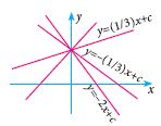
(i) m is an arbitrary constant
y = mx + c ...(1)
Differentiating w.r. to x ,
we get \(\frac{dy}{dx}\) = m  ...(2)
Now we eliminate m from (1) and (2)
For this substitute (2) in (1)
y = x \(\frac{dy}{dx}\) + c
x \(\frac{dy}{dx}\) - y + c = 0 which is the required differential equation of first order

(ii) c is an arbitrary constant
Differentiating (1), we get \(\frac{dy}{dx}\) = m
Here c is eliminated from the given equation
∴ \(\frac{dy}{dx}\) = m is the required differential equation.

(iii) both m and c are arbitrary constants
Since m and c are two arbitrary constants differentiating (1) twice we get
\(\frac{dy}{dx}\) = m
\(​​\frac { { d }^{ 2 }y }{ { dx }^{ 2 } } \) = 0
Here m and c are eliminated from the given equation.
\(​​\frac { { d }^{ 2 }y }{ { dx }^{ 2 } } \) = 0 which is the required differential equation.