
 100% FREE ACCESS
12th Standard Syllabus & Materials
12th Standard
TN 12th Computer Applications மின்னணு தரவு பரிமாற்றம் Sample Question Papers Study Material - QB365 Set A
NEW12th Standard
TN 12th Computer Applications மின் - வணிக பாதுகாப்பு அமைப்புகள் Sample Question Papers Study Material - QB365 Set A
NEW12th Standard
TN 12th Computer Applications மின்னணு செலுத்தல் முறைகள் Sample Question Papers Study Material - QB365 Set A
NEW12th Standard
TN 12th Computer Applications மின் - வணிகம் Sample Question Papers Study Material - QB365 Set A
NEW12th Standard
TN 12th Computer Applications திறந்த மூல கருத்துருக்கள் Sample Question Papers Study Material - QB365 Set A
NEW12th Standard
TN 12th Computer Applications வலையமைப்பு வடமிடல் Sample Question Papers Study Material - QB365 Set A

Published on: 30/09/2020
12th Standard Business Maths English Medium Important 5 Mark Book Back Questions (New Syllabus 2020)
Download Tamil Nadu 12th Standard Business Maths and Statistics question papers, model tests, one-mark questions, important questions, and public exam papers in PDF format. Free study materials and answer keys for TN State Board students.
Questions + Answers key
Take MCQ Business Maths and Statistics Test
1.
Solve the following equation by using Cramer’s rule
x + 4y + 3z = 2, 2x−6y + 6z = −3, 5x− 2y + 3z = −5
2.
Using Lagrange’s interpolation formula find a polynomial which passes through the points (0, –12), (1, 0), (3, 6) and (4,12).
3.
Using interpolation estimate the output of a factory in 1986 from the following data
| Year | 1974 | 1978 | 1982 | 1990 |
| Output in 1000 tones | 25 | 60 | 80 | 170 |
4.
The following data are taken from the steam table
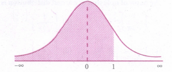
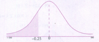
| Temperature C0 | 140 | 150 | 160 | 170 | 180 |
| Pressure kg f / cm2 | 3.685 | 4.854 | 6.302 | 8.076 | 10.225 |
Find the pressure at temperature t = 1750
5.
Using Newton’s formula for interpolation estimate the population for the year 1905 from the table:
| Year | 1891 | 1901 | 1911 | 1921 | 1931 |
| Population | 98.752 | 1,32,285 | 1,68,076 | 1,95,690 | 2,46,050 |
6.
A departmental head has four subordinates and four tasks to be performed. The subordinates differ in efficiency and the tasks differ in their intrinsic difficulty. His estimates of the time each man would take to perform each task is given below :
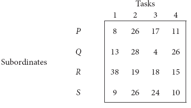
How should the tasks be allocated to subordinates so as to minimize the total man-hours?
7.
Solve (x2 + y2)dx + 2xy dy = 0
8.
Solve the following differential equations (3D2 + D − 14)y = 13e2x
9.
(D2 − 3D + 2)y = e3x which shall vanish for x = 0 and for x = log 2
10.
The following data gives the average life(in hours) and range of 12 samples of 5 lamps each. The data are
| Sample No | 1 | 2 | 3 | 4 | 5 | 6 |
| Sample Mean | 1080 | 1390 | 1460 | 1380 | 1230 | 1370 |
| Sample Range | 410 | 670 | 180 | 320 | 690 | 450 |
| Sample No | 7 | 8 | 9 | 10 | 11 | 12 |
| Sample Mean | 1310 | 1630 | 1580 | 1510 | 1270 | 1200 |
| Sample Range | 380 | 350 | 270 | 660 | 440 | 310 |
Construct control charts for mean and range. Comment on the control limits.
11.
Fit a straight line trend by the method of least squares to the following data.
| Year | 1980 | 1981 | 1982 | 1983 | 1984 | 1985 | 1986 | 1987 |
| Sales | 50.3 | 52.7 | 49.3 | 57.3 | 56.8 | 60.7 | 62.1 | 58.7 |
12.
Solve the following:
\(\frac{d y}{d x}+\frac{3 x^{2}}{1+x^{3}} y=\frac{1+x^{2}}{1+x^{3}}\)
13.
Construc \(\overset {-}{X}\) and R charts for the following data:
| Sample Number | Observations | ||
| 1 | 32 | 36 | 42 |
| 2 | 28 | 32 | 40 |
| 3 | 39 | 52 | 28 |
| 4 | 50 | 42 | 31 |
| 5 | 42 | 45 | 34 |
| 6 | 50 | 29 | 21 |
| 7 | 44 | 52 | 35 |
| 8 | 22 | 35 | 44 |
( Given for n = 3, A2 = 0.58,D3 = 0 and D4 = 2.115)
14.
Solve (x2 + 1)\(\frac { dy }{ dx } \) + 2xy = 4x2
15.
Calculate price index number for 2005 by
(a) Laspeyre’s
(b) Paasche’s method
| Commodity | 1995 | 2005 | ||
| Price | Quantity | Price | Quantity | |
| A | 5 | 60 | 15 | 70 |
| B | 4 | 20 | 8 | 35 |
| C | 3 | 15 | 6 | 20 |
16.
Solve the following homogeneous differential equations.
\(x\frac { dy }{ dx } -y=\sqrt { { x }^{ 2 }+{ y }^{ 2 } } \)
17.
The sales of a commodity in tones varied from January 2010 to December 2010 as follows:
| In year 2010 | Jan | Feb | Mar | Apr | May | Jun | Jul | Aug | Sep | Oct | Nov | Dec |
| Sales (in tones) | 280 | 240 | 270 | 300 | 280 | 290 | 210 | 200 | 230 | 200 | 230 | 210 |
Fit a trend line by the method of semi-average.
18.
If the marginal cost of producing x shoes is given by (3xy + y2)dx + (x2 + xy)dy = 0 and the total cost of producing a pair of shoes is given by Rs. 12. Then find the total cost function.
19.
20.
Construct Fisher’s price index number and prove that it satisfies both Time Reversal Test and Factor Reversal Test for data following data.
| Commodities | Base Year | Current Year | ||
| Price | Quantity | Price | Quantity | |
| Rice | 40 | 5 | 48 | 4 |
| Wheat | 45 | 2 | 42 | 3 |
| Rent | 90 | 4 | 95 | 6 |
| Fuel | 85 | 3 | 80 | 2 |
| Transport | 50 | 5 | 65 | 8 |
| Miscellaneous | 65 | 1 | 72 | 3 |
21.
Solve : x - y \(\frac { dx }{ dy } =a\left( { x }^{ 2 }+\frac { dx }{ dy } \right) \)
22.
23.
A sample of 100 students are drawn from a school. The mean weight and variance of the sample are 67.45 kg and 9 kg. respectively. Find
(a) 95% and
(b) 99% confidence intervals for estimating the mean weight of the students.
24.
Evaluate the following integrals:
\(\int _{ 0 }^{ 3 }{ \frac { xdx }{ \sqrt { x+1 } +\sqrt { 5x+1 } } } \)
25.
Explain in detail about simple random sampling with a suitable example.
26.
Evaluate the following integrals as the limit of the sum:
\(\int _{ 0 }^{ 1 }{ (x+4) } \)dx
27.
An auto company decided to introduce a new six cylinder car whose mean petrol consumption is claimed to be lower than that of the existing auto engine. It was found that the mean petrol consumption for the 50 cars was 10 km per litre with a standard deviation of 3.5 km per litre. Test at 5% level of significance, whether the claim of the new car petrol consumption is 9.5 km per litre on the average is acceptable.
28.
Evaluate \(\int _{ 2 }^{ 5 }{ \frac { \sqrt { x } }{ \sqrt { x } +\sqrt { 7-x } } } \) dx
29.
Using the following random number table,
| Tippet’s random number table | |||||||
| 2952 | 6641 | 3992 | 9792 | 7969 | 5911 | 3170 | 5624 |
| 4167 | 9524 | 1545 | 1396 | 7203 | 5356 | 1300 | 2693 |
| 2670 | 7483 | 3408 | 2762 | 3563 | 1089 | 6913 | 7991 |
| 0560 | 5246 | 1112 | 6107 | 6008 | 8125 | 4233 | 8776 |
| 2754 | 9143 | 1405 | 9025 | 7002 | 6111 | 8816 | 6446 |
Draw a sample of 10 children with their height from the population of 8,585 children as classified here under.
| Height (cm) | 105 | 107 | 109 | 111 | 113 | 115 | 117 | 119 | 121 | 123 | 125 |
| Number of children | 2 | 4 | 14 | 41 | 83 | 169 | 394 | 669 | 990 | 1223 | 1329 |
| Height(cm) | 127 | 129 | 131 | 133 | 135 | 137 | 139 | 141 | 143 | 145 | |
| No. of children | 1230 | 1063 | 646 | 392 | 202 | 79 | 32 | 16 | 5 | 2 |
30.
Time taken by a construction company to construct a flyover is a normal variate with mean 400 labour days and standard deviation of 100 labour days. If the company promises to construct the flyover in 450 days or less and agree to pay a penalty of Rs. 10,000 for each labour day spent in excess of 450. What is the probability that
(i) the company pays a penalty of atleast Rs. 2,00,000?
(ii) the company takes at most 500 days to complete the flyover?
31.
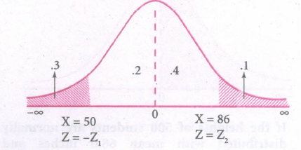
In a distribution 30% of the items are under 50 and 10% are over 86. Find the mean and standard deviation of the distribution.
32.
A car hiring firm has two cars. The demand for cars on each day is distributed as a Poisson variate, with mean 1.5. Calculate the proportion of days on which
(i) Neither car is used
(ii) Some demand is refused
33.
34.
A bank manager has observed that the length of time the customers have to wait for being attended by the teller is normally distributed with mean time of 5 minutes and standard deviation of 0.6 minutes. Find the probability that a customer has to wait
(i) for less than 6 minutes
(ii) between 3.5 and 6.5 minutes
35.
If X is a normal variate with mean 30 and SD 5. Find the probabilities that
(i) 26 ≤ X ≤ 40
(ii) X > 45
36.
If the average rain falls on 9 days in every thirty days, find the probability that rain will fall on atleast two days of a given week.
37.
The probability density function of a continuous random variable X is
\(f(x)=\left\{\begin{array}{l} a+b x^{2}, 0 \leq x \leq 1 \\ 0, \text { otherwise } \end{array}\right.\)
where a and b are some constants. Find
(i) a and b if E(X)\(\frac{3}{5}\)
(ii) Var(X).
38.
Integrate the following with respect to x.
ex (1+ x) log(xex)
39.
The demand equation for a product is pd = 20 − 5x and the supply equation is ps = 4x + 8. Determine the consumer’s surplus and producer’s surplus under market equilibrium.
40.
Determine the mean and variance of the random variable X having the following probability distribution.
| X=x | 1 | 2 | 3 | 4 | 5 | 6 | 7 | 8 | 9 | 10 |
| P(x) | 0.15 | 0.10 | 0.10 | 0.01 | 0.08 | 0.01 | 0.05 | 0.02 | 0.28 | 0.20 |
41.
The marginal cost of production of a firm is given by C'(x) = 5 + 0.13x, the marginal revenue is given by R'(x) = 18 and the fixed cost is Rs. 120. Find the profit function.
42.
The distribution of a continuous random variable X in range (–3, 3) is given by p.d.f.
\(f(x)=\left\{\begin{array}{l} \frac{1}{16}(3+x)^{2},-3 \leq x \leq-1 \\ \frac{1}{16}\left(6-2 x^{2}\right),-1 \leq x \leq 1 \\ \frac{1}{16}(3-x)^{2}, 1 \leq x \leq 3 \end{array}\right.\)
Verify that the area under the curve is unity.
43.
When the Elasticity function is \(\frac { x }{ x-2 } \). Find the function when x = 6 and y = 16.
44.
The marginal cost C'(x) and marginal revenue R'(x) are given by C'(x) = 50 + \(\frac{x}{50}\) and R'(x) = 60. The fixed cost is Rs. 200. Determine the maximum profit
45.
46.
Integrate the following with respect to x.
\(\frac { { 4x }^{ 2 }+2x+6 }{ { \left( x+1 \right) }^{ 2 }\left( x-3 \right) } \)
47.
Solve the equations x + 2y + z = 7, 2x − y + 2z = 4, x + y − 2z = −1 by using Cramer’s rule
48.
Two types of soaps A and B are in the market. Their present market shares are 15% for A and 85% for B. Of those who bought A the previous year, 65% continue to buy it again while 35% switch over to B. Of those who bought B the previous year, 55% buy it again and 45% switch over to A. Find their market shares after one year and when is the equilibrium reached?
49.
An automobile company uses three types of Steel S1, S2 and S3 for providing three different types of Cars C1, C2 and C3. Steel requirement R (in tonnes) for each type of car and total available steel of all the three types are summarized in the following table.
| Types of Steel | Types of Car | Total Steel available | ||
| C1 | C2 | C3 | ||
| S1 | 3 | 2 | 4 | 28 |
| S2 | 1 | 1 | 2 | 13 |
| S3 | 2 | 2 | 2 | 14 |
Determine the number of Cars of each type which can be produced by Cramer’s rule.
50.
The price of three commodities X, Y and Z are x, y and z respectively Mr. Anand purchases 6 units of Z and sells 2 units of X and 3 units of Y. Mr. Amar purchases a unit of Y and sells 3 units of X and 2units of Z. Mr. Amit purchases a unit of X and sells 3 units of Y and a unit of Z. In the process they earn Rs. 5,000/-, Rs. 2,000/- and Rs. 5,500/- respectively. Find the prices per unit of three commodities by rank method.
51.
Investigate for what values of ‘a’ and ‘b’ the following system of equations x + y + z = 6,x + 2y + 3z = 10, x + 2y + az = b have
(i) no solution
(ii) a unique solution
(iii) an infinite number of solutions.
52.
Show that the equations x + y + z = 6, x + 2y + 3z = 14, x + 4y + 7z = 30 are consistent and solve them.
53.
Construct the cost of living Index number for 2015 on the basis of 2012 from the following data using family budget method.
| Commodity | Price | Weight | |
| 2012 | 2015 | ||
| Rice | 250 | 280 | 10 |
| Wheat | 70 | 280 | 5 |
| Corn | 150 | 170 | 6 |
| Oil | 25 | 35 | 4 |
| Dhal | 85 | 90 | 3 |
54.
Evaluate \(\int _{ 0 }^{ \frac { \pi }{ 2 } }\) x sin x dx
55.
Evaluate \(\int _{ -1 }^{ 1 }{ { ({ x }^{ 3 }+{ 3x }^{ 2 }) }^{ 3 } } \) (x2 + 2x)dx
1.
\(\Delta =\left| \begin{matrix} 1 & 4 & 3 \\ 2 & -6 & 6 \\ 5 & -2 & 3 \end{matrix} \right| \)
= \(1\left| \begin{matrix} -6 & 6 \\ -2 & 3 \end{matrix} \right| -4\left| \begin{matrix} 2 & 6 \\ 5 & 3 \end{matrix} \right| +3\left| \begin{matrix} 2 & -6 \\ 5 & -2 \end{matrix} \right| \)
= 1(-18 + 12) - 4(6 - 30) +3 (- 4 +30)
= 1(- 6) - 4(- 24) + 3(26)
= - 6 + 96 + 78 = 168 \(\neq \) 0
Since \(\Delta \neq 0\) the system is consistent with unique solution and Cramer's rule can be applied
\(\Delta x=\left| \begin{matrix} 2 & 4 & 3 \\ -3 & -6 & 6 \\ -5 & -2 & 3 \end{matrix} \right| \)
= \(2\left| \begin{matrix} -6 & 6 \\ -2 & 3 \end{matrix} \right| -4\left| \begin{matrix} -3 & 6 \\ -5 & 3 \end{matrix} \right| +3\left| \begin{matrix} -3 & -6 \\ -5 & -2 \end{matrix} \right| \)
= 2 (- 18 + 12) - 4(- 9 +30) + 3(6 -30)
= 2(- 6) - 4(21) + 3(- 24)
= -12-84-72 =-168
\(\Delta y=\left| \begin{matrix} 1 & 2 & 3 \\ 2 & - & 6 \\ 5 & -5 & 3 \end{matrix} \right| =1\left| \begin{matrix} -3 & 6 \\ -5 & 3 \end{matrix} \right| -2\left| \begin{matrix} 2 & 6 \\ 5 & 3 \end{matrix} \right| +3\left| \begin{matrix} 2 & -3 \\ 5 & -5 \end{matrix} \right| \)
= 1 (-9+30)-2(6-30)+3(- 10+ 15)
= 1(21) - 2(- 24) + 3(5)
= 21 + 48 + 15 = 84
\(\Delta z=\left| \begin{matrix} 1 & 4 & 2 \\ 2 & -6 & -3 \\ 5 & -2 & -5 \end{matrix} \right| \)
= \(1\left| \begin{matrix} -6 & -3 \\ -2 & -5 \end{matrix} \right| -4\left| \begin{matrix} 2 & -3 \\ 5 & -5 \end{matrix} \right| +2\left| \begin{matrix} 2 & -6 \\ 5 & -2 \end{matrix} \right| \)
= 1(30-6)-4(-10+ 15)+2(-4+30)
= 24 - 4(5) + 2(26)
= 24 - 20 + 52 = 56
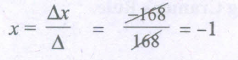
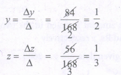
Solution set is \(\left\{ -1,\frac { 1 }{ 2 } ,\frac { 1, }{ 3 } \right\} \)
2.
Given
| x | 0 | 1 | 3 | 4 |
| y | -12 | 0 | 6 | 12 |
Here the intervals are unequal
∴ By Lagranges interpolation formula, we have
x0 = 0, x1 = 1, x2 = 3, x3 = 4
y0 = -12, y1 = 0, y2 = 6, y3 = 12 and x = x.
∴ y = f(x) = \(\frac { (x-{ x }_{ 1 })(x-{ x }_{ 2 })(x-{ x }_{ 3 }) }{ ({ x }_{ 0 }-{ x }_{ 1 })({ x }_{ 0 }-{ x }_{ 2 })({ x }_{ 0 }-{ x }_{ 3 }) } \times { y }_{ 0 }+\frac { (x-{ x }_{ 0 })(x-{ x }_{ 2 })(x-{ x }_{ 3 }) }{ ({ x }_{ 1 }-{ x }_{ 0 })({ x }_{ 1 }-{ x }_{ 2 })(x_{ 1 }-{ x }_{ 3 }) } \times { y }_{ 1 }+\frac { (x-{ x }_{ 0 })(x-{ x }_{ 1 })(x-{ x }_{ 3 }) }{ ({ x }_{ 2 }-{ x }_{ 0 })({ x }_{ 2 }-{ x }_{ 1 })({ x }_{ 2 }-{ x }_{ 3 }) } \times { y }_{ 2 }+\frac { (x-{ x }_{ 0 })(x-{ x }_{ 1 })(x-{ x }_{ 2 }) }{ ({ x }_{ 3 }-{ x }_{ 0 })({ x }_{ 3 }-{ x }_{ 1 })({ x }_{ 3 }-{ x }_{ 2 }) } \times { y }_{ 3 }\)
= \(\frac { (x-1)(x-3)(x-4) }{ (0-1)(0-3)(0-4) } (-12)+\frac { (x-0)(x-3)(x-4) }{ (1-0)(1-3)(1-4) } (0)+\frac { (x-0)(x-1)(x-4) }{ (3-0)(3-1)(3-4) } (6)+\frac { (x-1)(x-3)(x-4) }{ (4-0)(4-1)(4-3) } (12)\)
= \(\frac { (x-1)(x-3)(x-4) }{ (-1)(-3)(-4) } (-12)+0+\frac { x(x-1)(x-4) }{ (3)(2)(-1) } (6)+\frac { x(x-1)(x-3) }{ (4)(3)(1) } (12)\)
= +[(x - 1)(x - 3)(x - 4)] - x (x - 1)(x - 4) + x(x - 1)(x - 3)
= +[(x3-4x+3)(x-4)] -x(x2-5x+4) + x(x2-4x + 3)
= - (x3 - 8x2+ 19x - 12) - 4x2 + 3x
= (x - 4)(x2 - 4x + 3) - x (x2 - 5x + 4) + x(x2 - 4x + 3)

= x3 - 7x2 + 19x - 12.
3.
Given
| Year | 1974 | 1978 | 1982 | 1990 |
| Output in 1000 tones | 25 | 60 | 80 | 170 |
Here the intervals are unequal.
∴ By Lagranges interpolation formula, we have
x0 = 1974, x1 = 1978, x2 = 1982, x3 = 1990
y0 = 25, y1 = 60, y2 = 80, y3 = 170 and x = 1986.
∴ y = f(x) = \(\frac { (x-{ x }_{ 1 })(x-{ x }_{ 2 })(x-{ x }_{ 3 }) }{ ({ x }_{ 0 }-{ x }_{ 1 })({ x }_{ 0 }-{ x }_{ 2 })({ x }_{ 0 }-{ x }_{ 3 }) } \times { y }_{ 0 }+\frac { (x-{ x }_{ 0 })(x-{ x }_{ 2 })(x-{ x }_{ 3 }) }{ ({ x }_{ 1 }-{ x }_{ 0 })({ x }_{ 1 }-{ x }_{ 2 })(x_{ 1 }-{ x }_{ 3 }) } \times { y }_{ 1 }+\frac { (x-{ x }_{ 0 })(x-{ x }_{ 1 })(x-{ x }_{ 3 }) }{ ({ x }_{ 2 }-{ x }_{ 0 })({ x }_{ 2 }-{ x }_{ 1 })({ x }_{ 2 }-{ x }_{ 3 }) } \times { y }_{ 2 }+\frac { (x-{ x }_{ 0 })(x-{ x }_{ 1 })(x-{ x }_{ 2 }) }{ ({ x }_{ 3 }-{ x }_{ 0 })({ x }_{ 3 }-{ x }_{ 1 })({ x }_{ 3 }-{ x }_{ 2 }) } \times { y }_{ 3 }\)
\(\frac { (x-{ x }_{ 0 })(x-{ x }_{ 2 })(x-{ x }_{ 3 }) }{ ({ x }_{ 0 }-{ x }_{ 1 })({ x }_{ 0 }-{ x }_{ 2 })({ x }_{ 0 }-{ x }_{ 3 }) } \times25+\frac { (x-{ x }_{ 0 })(x-{ x }_{ 2 })(x-{ x }_{ 3 }) }{ ({ x }_{ 1 }-{ x }_{ 0 })({ x }_{ 1 }-{ x }_{ 2 })(x_{ 1 }-{ x }_{ 3 }) } \times60+\frac { (x-{ x }_{ 0 })(x-{ x }_{ 1 })(x-{ x }_{ 3 }) }{ ({ x }_{ 2 }-{ x }_{ 0 })({ x }_{ 2 }-{ x }_{ 1 })({ x }_{ 2 }-{ x }_{ 3 }) } \times80+\frac { (x-{ x }_{ 0 })(x-{ x }_{ 1 })(x-{ x }_{ 2 }) }{ ({ x }_{ 3 }-{ x }_{ 0 })({ x }_{ 3 }-{ x }_{ 1 })({ x }_{ 3 }-{ x }_{ 2 }) } \times 70+\frac { (1986-1974)(1986-1982)(1986-1990) }{ (1990-1974)(1990-1978)(1990-1982) } \times 170\)
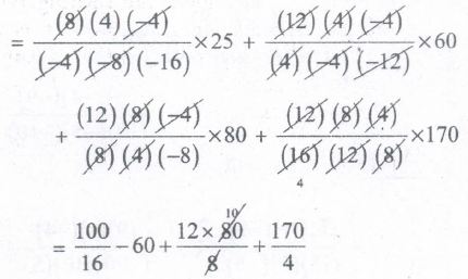
= 6.25 - 60 + 120 + 42.5
y = 108.75
4.
Since the pressure required is at the end of the table, we apply Backward interpolation formula. Let temperature be x and the pressure be y.
\({ y }_{ \left( x={ x }_{ 0 }+nh \right) }={ y }_{ 0 }+\frac { n }{ n! } \Delta { y }_{ 0 }+\frac { n(n-1) }{ 2! } { \Delta }^{ 2 }{ y }_{ 0 }+\frac { n(n-)(n-2) }{ 3! } { \Delta }^{ 3 }{ y }_{ 0 }+...\)
To find y at x = 175
\(\therefore\) xn + nh = 175 , xn = 180, h = 10 \(\Rightarrow\) n = −0.5
| x | y | \(\Delta y\) | \(\Delta ^{ 2 }y\) | \(\Delta ^{ 2 }y\) | \(\Delta ^{ 4 }y\) |
| 140 | 3.685 | ||||
| 1.169 | |||||
| 150 | 4.854 | 0.279 | |||
| 1.448 | 02.047 | ||||
| 160 | 6.032 | 0.326 | 0.002 | ||
| 1.774 | 0.049 | ||||
| 170 | 8.076 | 0.375 | |||
| 2.149 | |||||
| 180 | 10.225 |
\({ y }_{ (x=1750 }=10.225+\left( -0.5 \right) (2.149)+\frac { (-0.5)(0-5) }{ 2! } (0.375)+\frac { (-0.5)(0-5)(1.5) }{ 3! } (0.049)+\frac { (-0-5)(0.5)(1.5)(2.5) }{ 4! } (0.002)\)
= 10.225−1.0745−0.046875−0.0030625 − 0.000078125
= 9.10048438
= 9.1
5.
To find the population for the year 1905 (i.e) the value of y at x = 1905
Since the value of y is required near the beginning of the table, we use the Newton’s forward interpolation formula.
\({ y }_{ \left( x={ x }_{ 0 }+nh \right) }={ y }_{ 0 }+\cfrac { n }{ n! } \Delta { y }_{ 0 }+\cfrac { n(n-1) }{ 2! } { \Delta }^{ 2 }{ y }_{ 0 }+\cfrac { n(n-)(n-2) }{ 3! } { \Delta }^{ 3 }{ y }_{ 0 } + ...\)
To find y at x = 1905
\(\therefore\) x0+nh = 1905 , x0 = 1891, h = 10
1891+n(10) = 1905 \(\Rightarrow\) n = 1.4
| x | y | \(\Delta y\) | \(\Delta ^{ 2 }y\) | \(\Delta ^{ 3 }y\) | \(\Delta ^{ 4 }y\) |
|---|---|---|---|---|---|
| 1891 | 98,752 | ||||
| 33,533 | |||||
| 1901 | 1,32,285 | 2,258 | |||
| 35,791 | –10,435 | ||||
| 1911 | 1,68,076 | -8,177 | 41,376 | ||
| 27,614 | |||||
| 1921 | 1,95,690 | 30,941 | |||
| 22,764 | |||||
| 50,360 | |||||
| 1931 | 2,46,050 |
y(x=1905) = \(98,752+(1.4)(33533)+\frac { (1.4)(0.4) }{ 2 } (2258)+\frac { (1.4)(0.4)(-0.6) }{ 6 } (-10435)+\frac { (1.4)(0.6)(-0.6)(-1.6) }{ 24 } (41358)\)
= 98,752 + 46946.2 + 632.4 + 584.36 + 1389.63
= 1,48,304.43
= 1,48,304
6.
Here the number of rows and columns are equal
∴ The given assignment problem is balanced.
Step 1 : Select a minimum element in each row and subtract this from all the elements in its row.
∴ The cost matrix of the given assignment problem is
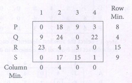
Column 2 has no zero. Go to Step 2.
Step 2 : Select the minimum element in each column and subtract this from all the elements in its column.
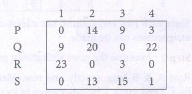
Since each row and column contains atleast one zero, assignments can be made.
Step 3 : Examine the rows with exactly one zero, mark it by and draw a vertical line.
After examining the rows, examine the columns with exactly one zero.
Mark it by and draw a horizontal line.
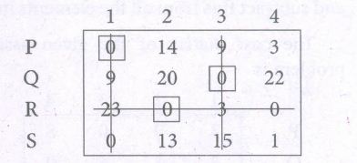
Only 3 assignments have been made.
The numbers not lying on the line are and min. is 1. Subtract 1 from all these numbers and add 1 to 23 which lies on the intersecting lines. Other numbers remain the same.
A new cost matrix is formed and repeat step 3.
∴ The new cost matrix is
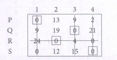
Thus, all the 4 assignments have been made.
∴The optimal assignment schedule and total cost is
| Subordinates | tasks | cost |
|---|---|---|
| P | 1 | 8 |
| Q | 3 | 4 |
| R | 2 | 19 |
| S | 4 | 10 |
| Total Cost | Rs. 41 | |
7.
(x2 +y2) dx = -2xy dy
⇒ \(\frac { dy }{ dx } =-\frac { ({ x }^{ 2 }+{ { y }^{ 2 }) } }{ 2xy } \)
Since the numerator and denominator is a homogenous function of degree 2,
put y = vx and \(\frac { dy }{ dx } =v+x\frac { dy }{ dx } \)
x\(\frac { dv }{ dx } =-\left( \frac { { x }^{ 2 }+{ v }^{ 2 }{ x }^{ 2 } }{ 2xvx } \right) \)
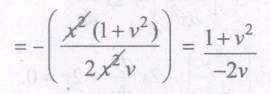
x\(\frac { dv }{ dx } =-\left( \frac { 1+{ v }^{ 2 } }{ 2v } \right) -v\)
= \(\frac { -1-{ v }^{ 2 }-2{ v }^{ 2 } }{ 2v } -\frac { -1-3{ v }^{ 2 } }{ 2v } =-\left( \frac { 1+3{ v }^{ 2 } }{ 2v } \right) \)
\(\frac { 2v.dv }{ 1+3{ v }^{ 2 } } =-\frac { dx }{ x } \)
Multiplying by 3,
put 1 + 3v2 = t
6v dv = dt
\(\int { \frac { 6vdv }{ 1+3v^{ 2 } } } dv=-\int { 3 } \frac { dx }{ x } \)
\(\int { \frac { dt }{ t } } =-3\int { \frac { dx }{ x } } \)
⇒ log t = - 3 log x + log C
⇒ log (1 + 3v2) + 3 log x = log C
⇒ log (1 + 3v2) .x3 = log C
⇒ (1 + 3v2)x3= C
Replace v by \(\frac { y }{ x } \) we get,
\(\left( 1+\frac { { 3y }^{ 2 } }{ { x }^{ 2 } } \right) \).x3= C
⇒ \(\left( 1+\frac { { 3y }^{ 2 } }{ { x }^{ 2 } } \right) ^{ \frac { 1 }{ 3 } }\)= C
8.
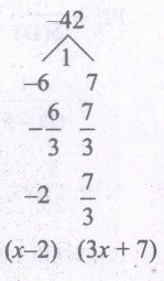
The auxiliary equation is 3m2 + m -14 = 0
(m-2)\(\frac { 7 }{ 3 } \) = 0
⇒ m = 2, -\(\frac { 7 }{ 3 } \)
The roots are real and different
∴ CF is Ae2x+\(Be^{ -\frac { 7 }{ 3 } x }\)
Particular Integral PI = \(\frac { 1 }{ \phi (D) } \).f(x)
PI = \(\frac { 1 }{ (3D^{ 2 }+D-14) } \).13 e2x
= \(\frac { 13.e^{ 2x } }{ 3D^{ 2 }+D-14 } \)
= \(\frac { 13e^{ 2x } }{ (D-2)(3D+7) } =\frac { 13e^{ 2x } }{ 3(D-2)\left( D+\frac { 7 }{ 3 } \right) } \)
= \(\frac { 13x{ e }^{ 2x } }{ 3\left( 2+\frac { 7 }{ 3 } \right) } \)
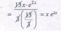
∴ y = CF + PI
∴ The general solution is
y = Ae2x+\({ Be }^{ -\frac { 7 }{ 3 } x }\) + xe2x
9.
Auxiliary equation is m2 - 3m + 2 = 0
∴ (m - 1)(m - 2) = 0
⇒ m = 1,2
∴ Complementary function CF is Aex + Be2x
PI = \(\frac { 1 }{ \phi (D) } \)(x)
= \(\frac { 1 }{ { D }^{ 2 }-3D+2 } \).e3x
= \(\frac { 1 }{ (D-1)(D-2) } \).e3x
= \(\frac { e^{ 3x } }{ (3-1)(3-2) } \).e3x
= \(\frac { { e }^{ 3x } }{ 2 } \)
General solution is y = CF + PI
y = Aex+Be2x+\(\frac { 1 }{ 2 } \)e3x ...(1)
Given when x = 0, y = 0
∴ 0 = Ae0+Be0+\(\frac { 1 }{ 2 } \)e0 ⇒ 0 = A+B-\(\frac { 1 }{ 2 } \) ..(2)
Also, when x = log2, y = 0
⇒ 0 = Aelog2+Be2log2+e3log3
⇒ 0 = A(2)+\(Be^{ log2^{ 2 }+ }+\frac { 1 }{ 2 } elog2^{ 3 }\)
⇒ 0 = 2A+4B+\(\frac{8}{2}\) ⇒ 2A+4B=-4
⇒ A+2B = -2
(2)-(3) ⇒ A+B = -\(\frac { 1 }{ 2 } \)
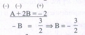
Substituting B = -\(\frac { 3 }{ 2 } \) in (2) we get
\(A-\frac { 3 }{ 2 } =-\frac { 1 }{ 2 } \Rightarrow A=-\frac { 1 }{ 2 } +\frac { 3 }{ 2 } \Rightarrow \frac { 2 }{ 2 } \)=1
∴ y = \(1.e^{ x }-\frac { 3 }{ 2 } e^{ 2x }+\frac { e^{ 3x } }{ 2 } \).
10.
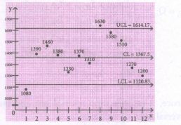
\(\overline {\overline{X}} = \frac {1080+1390+1460+1380+1230+1370+1310+1630+1580+1510+1270+1200}{12}\)
\(\overline {\overline{X}}\) = \(\frac {16410}{12}\) = 1367.5
\(\overline {\overline{R}} = \frac {410+670+180+320+690+450+380+350+270+660+440+310}{12}\)
\(\overline {R}\) = \(\frac {5130}{12}\) = 427.5
The control limits of mean chart are
UCL = \(\overline {\overline{X}} + A_{2} \overline{R}\)
= 1367.5 + 0.577(427.5)
= 1367.5 + 246.67 = 1614.17
CL = \(\overline {\overline{X}}\) = 1367.5
LCL = \(\overline {\overline{X}} - A_{2} \overline{R}\)
= 1367.5 - 246.67 = 1120.83
The control limits of range chart are
UCL = D4\(\overline {R}\) = 2.114 (427.5) = 903.74
CL = \(\overline {R}\) = 427.5
[For n=5, A2 = 0.577, D3 = 0, D4 = 2.114]
LCL = D3\(\overline {R}\) = 0
\(\overline {X}\) - chart

R-chart
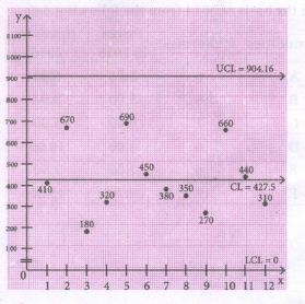
Conclusion: The above diagram shows all the control lines with the data points plotted.
Since one point in mean chart, lie outside the control limits, we can say that the process is out of control.
11.
| Year X | Sales Y | X = \(\frac {x-1983.5}{0.5}\) | XY | X2 |
| 1980 | 50.3 | -7 | -352.1 | 49 |
| 1981 | 52.7 | -5 | -263.5 | 25 |
| 1982 | 49.3 | -3 | -147.9 | 9 |
| 1983 | 57.3 | -1 | -57.3 | 1 |
| 1984 | 56.8 | 1 | 56.8 | 1 |
| 1985 | 60.7 | 3 | 182.1 | 9 |
| 1986 | 62.1 | 5 | 310.5 | 25 |
| 1987 | 58.7 | 7 | 410.9 | 49 |
| 447.9 | 0 | 139.5 | 168 |
Since \(\sum X = 0, a = \frac {\sum Y}{n} = \frac {447.9}{8} = 55.9875\)
b = \(\frac {\sum XY}{\sum X^{2}} = \frac{139.5}{168}\) = 0.83035
∴ The straight line trend is obtained by
Y = a + bX ⇒ Y = 55.9875 + 0.830 \((\frac {x-1983.5}{0.5})\)
= 55.9875 + 0.8304 (-5)
= 55.9875 - 4.152
= 51.8355
12.
The given differential equation is of this form
\(\frac { dy }{ dx } \)+Py = Q Where
P = \(\frac { 3x^{ 2 } }{ 1+{ x }^{ 3 } } \); Q=\(\frac { 1+x^{ 2 } }{ 1+{ x }^{ 3 } } \)
∴ \(\int { p } dx=\int { \frac { 3x^{ 2 } }{ 1+{ x }^{ 3 } } } \)dx
put t = 1+x3 ⇒ dt = 3x2 dx
=\(\int { \frac { dt }{ t } } \) = log t =log(1+x3) [∵ t = 1+x3]
∴ Integrating factor (I. F) = \(e^{ \int { p } dx }=e^{ log(1+x^{ 3 }) }\)
= 1 + x3
Hence the solution is
\(ye^{ \int { p } dx }=\int { Q } .e^{ \int { p } dx }dx+c\)

=\(\int { (1+{ x }^{ 2 }) } dx\) + c
⇒ y(1+x3) = x + \(\frac { { x }^{ 3 } }{ 3 } \) + c
13.
| Sample No | Observations | Total | \(\overline {X}\) | R = x max - xmin | ||
| 1 | 2 | 3 | ||||
| 1 | 32 | 36 | 42 | 110 | \(\frac {100}{3} = 36.7\) | 42-32 = 10 |
| 2 | 28 | 32 | 40 | 100 | \(\frac {100}{3} = 33.3\) | 40-28 = 12 |
| 3 | 39 | 52 | 28 | 119 | \(\frac {119}{3} = 39.7\) | 52 -28 = 24 |
| 4 | 50 | 42 | 31 | 123 | \(\frac {123}{3} = 41\) | 50-31 = 19 |
| 5 | 42 | 45 | 34 | 121 | \(\frac {123}{3} = 40.3\) | 45-34 = 29 |
| 6 | 50 | 29 | 21 | 100 | \(\frac {100}{3} = 33.3\) | 50-21 = 29 |
| 7 | 44 | 52 | 35 | 131 | \(\frac {131}{3} = 43.7\) | 52-35 = 17 |
| 8 | 22 | 35 | 44 | 101 | \(\frac {101}{3} = 33.7\) | 44-22 = 22 |
| 301.7 | 144 | |||||
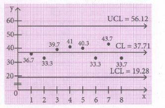
\(\overline {\overline{X}}\) = \(\frac {301.7}{8}\) = 37.71
\(\overline{R}\) = \(\frac {144}{8}\) = 18
Control limits for \(\overline {X}\) - chart
UCl = \(\overline {\overline{X}} + A_{2} \overline {R}\)
= 37.71 + 0.58 (18)
= 37.71 + 18.44
[when n = 3, A2 = 1.023]
UCL = 56.12
CL = \(\overline {\overline{X}}\) = 37.71
LCL = \(\overline {\overline{X}} - A_{2} \overline {R}\)
= 37.71 - 18.44
LCL = 19.28
Control limits for R-chart
UCL = D4 \(\overline {R}\) = 2.2574(18) = 46.33
CL = \(\overline {R}\) = 18
LC = D3 \(\overline {R}\) = 0
when n = 3, D4 = 2.574]
\(\overline {X}\) - chart
.\(\overline {R}\) - chart
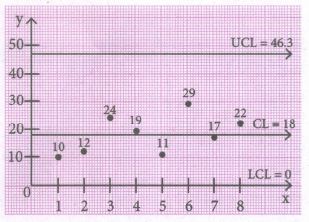
Conclusion: The above diagram shows all the control lines with the data points plotted. Since all the points lie within the control limits, we can say that the process is in control.
14.
The given equation can be reduced to
\(\frac { dy }{ dx } +\frac { 2x }{ { x }^{ 2 }+1 } y=\frac { 4{ x }^{ 2 } }{ { x }^{ 2 }+1 } \)
It is of the form \(\frac { dy }{ dx } \) + Py = Q
Here P \(=\frac { 2x }{ { x }^{ 2 }+1 } ,Q=\frac { 4{ x }^{ 2 } }{ { x }^{ 2 }+1 } \)
ഽPdx = ഽ\(\frac { 2x }{ { x }^{ 2 }+1 } \)dx = log(x2 +1)
I.F = eഽpdx = elog(x2+1) = x2 + 1
The required solution is y(IF) = ഽQ(I.F)dx + c
y(x2 +1) = ഽ\(\frac { 4{ x }^{ 2 } }{ { x }^{ 2 }+1 } \)(x2 + 1)dx + c
y(x2 +1) = \(\frac { 4{ x }^{ 3 } }{ 3 } \) + c
15.
| Commodity | 1995 | 2005 | ||
| Price(p0) | (q0) | Price | Quantity | |
| A | 5 | 60 | 15 | 70 |
| B | 4 | 20 | 8 | 35 |
| C | 3 | 15 | 6 | 20 |
| p0q0 | p0q1 | p1q0 | p1q1 |
| 300 | 350 | 900 | 1050 |
| 80 | 140 | 160 | 280 |
| 45 | 60 | 90 | 120 |
| 425 | 550 | 1150 | 1450 |
Laspeyre's price index number
\(P^{L}_{01}\) = \({\frac {\sum p_{1}q_{0}}{\sum p_{0}q_{0}}} \times 100\)
= \(\frac {1150}{425} \times {100}\) = 270.58
Paasche's index number
\(P^{L}_{01}\) = \({\frac {\sum p_{1}q_{0}}{\sum p_{0}q_{1}}} \times 100\)
= \(\frac {1450}{550} \times {100}\) = 263.63
16.
\(x\frac { dy }{ dx } =y+\sqrt { { x }^{ 2 }+{ y }^{ 2 } } \)
\(\frac { dy }{ dx } =\frac { \left[ y+\sqrt { { x }^{ 2 }+{ y }^{ 2 } } \right] }{ x } \)
Since the numerator and denominator is a homogeneous function of degree 1,
put y = vx and \(\frac { dy }{ dx } =v+x\frac { dv }{ dx } \)
∴ v + x\(\frac { dv }{ dx } =\frac { vx+\sqrt { { x }^{ 2 }+{ v }^{ 2 }{ x }^{ 2 } } }{ x } =\frac { vx+x\sqrt { 1+{ v }^{ 2 } } }{ x } \)
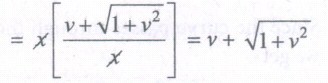
⇒ x\(\frac { dv }{ dx } =v+\sqrt { 1+{ v }^{ 2 } } -v=\sqrt { 1+v^{ 2 } } \)
Separating the variables we get,
\(\frac { dx }{ \sqrt { 1+{ v }^{ 2 } } } =\frac { dx }{ x } \)
Integrating both sides we get,
\(\int { \frac { dv }{ \sqrt { 1+{ v }^{ 2 } } } } =\int { \frac { dx }{ x } } \)
\(\left[ \therefore \int { \frac { dx }{ \sqrt { { x }^{ 2 }+a^{ 2 } } } } =log\left| x+\sqrt { { x }^{ 2 }+{ a }^{ 2 } } +c \right| \right] \)
⇒ \(log\left| v+\sqrt { { v }^{ 2 }+1 } \right| \) =log x + log c
⇒ \(log(v+\sqrt { { v }^{ 2 }+1 } )\) =log xc
⇒ v+\(\sqrt { { v }^{ 2 }+1 } \)= xc
Replace v by \(\frac { y }{ x } \) we get,
\(\frac { y }{ x } +\sqrt { \frac { { y }^{ 2 } }{ { x }^{ 2 } } +1 } \)= xc
⇒ \(\frac { y }{ x } +\sqrt { \frac { { x }^{ 2 }+{ y }^{ 2 } }{ x } } \)= xc
⇒ y+\(\\ \frac { y+\sqrt { \frac { { x }^{ 2 }+{ y }^{ 2 } }{ x } } }{ x } \)= xc
⇒ y+\(\sqrt { { x }^{ 2 }+{ y }^{ 2 } } \) = x2c
17.
| Year 2010 | Sales (in tones) |
|---|---|
| Jan | 280 |
| Feb | 240 |
| Mar | 270 |
| Apr | 300 |
| May | 280 |
| June | 290 |
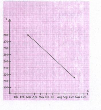
Average
\(\frac {280 + 240 + 270 + 300 + 280 + 290}{6}\) = \(\frac {1660}{6}\) = 276.6666
| Year 2010 | Sales (in tones) |
|---|---|
| Jul | 210 |
| Aug | 200 |
| Sep | 230 |
| Oct | 200 |
| Nov | 230 |
| Dec | 210 |
\(\frac {210+ 200+ 230+ 200+ 230+ 210}{6}\) = \(\frac {1280}{6}\) = 213.333
Since the number of years is even (12), we can equally divide the given data into two equal parts and obtain the averages of first 6 months and last 6 months.
18.
Given marginal cost function is (x2 + xy)dy + (3xy + y2)dx = 0
\(\frac { dy }{ dx } =\frac { -(3xy+{ y }^{ 2 }) }{ { x }^{ 2 }+xy } \) (1)
Put y = vx and \(\frac { dy }{ dx } =v+x\frac { dv }{ dx } \) in (1)
\(v+x\frac { dv }{ dx } =\frac { -(3xvx+{ v }^{ 2 }{ x }^{ 2 }) }{ { x }^{ 2 }+xvx } \)
\(=\frac { -(3v+{ v }^{ 2 }) }{ 1+v } \)
Now, \(x\frac { dv }{ dx } =\frac { -3v-{ v }^{ 2 } }{ 1+v } -v\)
\(=\frac { -3v-{ v }^{ 2 }-v-{ v }^{ 2 } }{ 1+v } \)
\(x\frac { dv }{ dx } =\frac { -4v-{ 2v }^{ 2 } }{ 1+v } \)
\(\frac { 1+v }{ 4v+2{ v }^{ 2 } } dv=\frac { -dx }{ x } \)
On Integration
\(\int { \frac { 1+v }{ 4v+2{ v }^{ 2 } } } =-\int { \frac { dx }{ x } } \)
Now, multiply 4 on both sides
\(\int { \frac { 1+v }{ 4v+2{ v }^{ 2 } } } =-4\int { \frac { dx }{ x } } \)
log (4v+2v2) = −4 logx+logc
4v + 2v2 = \(\frac { c }{ { x }^{ 4 } } \)
x4(4v + 2v2) = c
Replace \(v=\frac { y }{ x } \)
\({ x }^{ 4 }\left( 4\frac { y }{ x } +2\frac { { y }^{ 2 } }{ { x }^{ 2 } } \right) =c\)
\({ x }^{ 4 }\left[ \frac { 4xy+2{ y }^{ 2 } }{ { x }^{ 2 } } \right] \) = c
c = 2x2(2xy + y2) (2)
Cost of producing a pair of shoes = Rs. 12
(i.e) y = 12 when x = 2
c = 8[48 + 144]= 1536
∴ The cost function is x2(2xy + y2) = 768
19.
20.
| Commodities | Base Year | Current Year | p0q0 | p0q1 | p1q0 | p1q1 | ||
| Price (p0) |
Quantity (q1) |
Price ((p0)) |
Quantity (q1) |
|||||
| Rice | 40 | 5 | 48 | 4 | 200 | 160 | 240 | 192 |
| Wheat | 45 | 2 | 42 | 3 | 90 | 135 | 84 | 126 |
| Rent | 90 | 4 | 95 | 6 | 360 | 540 | 380 | 570 |
| Fuel | 85 | 3 | 80 | 2 | 255 | 170 | 240 | 160 |
| Transport | 50 | 5 | 65 | 8 | 250 | 400 | 325 | 520 |
| Miscellaneous | 65 | 1 | 72 | 3 | 65 | 195 | 72 | 216 |
| Total | 1220 | 1600 | 1341 | 1784 | ||||
Fisher’s price index number
\({ P }_{ 01 }^{ F }=\left( \sqrt { \frac { \sum { { p }_{ 1 }{ q }_{ 10 } } \times \sum { { p }_{ 1 }{ q }_{ 1 } } }{ \sum { { p }_{ 0 }{ q }_{ 0 } } \times \sum { { p }_{ 0 }{ q }_{ 1 } } } } \right) \times 100=\left( \sqrt { \frac { 1341\times 1784 }{ 1220\times 1600 } } \right) \times 100=110.706\)
Time Reversal Test:P01x P10=1
\({ P }_{ 01 }\times { P }_{ 10 }=\sqrt { \left( \frac { \sum { { p }_{ 1 }{ q }_{ 0 } } \times \sum { { p }_{ 1 }{ q }_{ 1 } } \times \sum { { p }_{ 0 }{ q }_{ 1 } } \times \sum { { p }_{ 0 }{ q }_{ 0 } } }{ \sum { { p }_{ 0 }{ q }_{ 0 } } \times \sum { { p }_{ 0 }{ q }_{ 1 } } \times \sum { { p }_{ 1 }{ q }_{ 1 } } \times \sum { { p }_{ 1 }{ q }_{ 0 } } } \right) } \)
\({ P }_{ 01 }\times { P }_{ 10 }=\sqrt { \left( \frac { 1341\times 1784\times 1600\times 1220 }{ 1220\times 1600\times 1784\times 1341 } \right) } \)
P01x P10 = 1
Factor Reversal Test
\(P_{01} \times Q_{01}=\frac{\sum p_{1} q_{1}}{\sum p_{0} q_{0}}\)
\(P_{01} \times Q_{01}=\sqrt{\left(\frac{\sum p_{1} q_{0} \times \sum p_{1} q_{1} \times \sum q_{1} p_{0} \times \sum q_{1} p_{1}}{\sum p_{0} q_{0} \times \sum p_{0} q_{1} \times \sum q_{0} p_{0} \times \sum q_{0} p_{1}}\right)}\)
\(P_{01} \times Q_{01}=\sqrt{\left(\frac{1341 \times 1784 \times 1600 \times 1784}{1220 \times 1600 \times 1220 \times 1341}\right)}\)
\(P_{01} \times Q_{01}=\sqrt{\left(\frac{1784 \times 1784}{1220 \times 1220}\right)}=\frac{1784}{1220}\)
\(\Rightarrow P_{01} \times Q_{01}=\frac{\sum p_{1} q_{1}}{\sum p_{0} q_{0}}\)
21.
Given x - y \(\frac { dx }{ dy } =a\left( { x }^{ 2 }+\frac { dx }{ dy } \right) \)
\(x-y\frac { dx }{ dy } ={ ax }^{ 2 }+a\frac { dx }{ dy } \)
\(x-{ ax }^{ 2 }=a\frac { dx }{ dy } +y\frac { dx }{ dy } \)
x(1 − ax) = (a + y)\(\frac { dx }{ dy } \)
By separating the variables, we get
\(\frac { dx }{ x(1-ax) } =\frac { dy }{ a+y } \)
\(\left( \frac { a }{ 1-ax } +\frac { 1 }{ x } \right) dx=\frac { dy }{ a+y } \)
Integrating, ഽ\(\left( \frac { a }{ 1-ax } +\frac { 1 }{ x } \right) dx=\frac { dy }{ a+y } \)
−log(1 − ax) + log x = log(a + y) + logc
\(log\left( \frac { x }{ 1-ax } \right) \) = log(c(a + y))
\(\left( \frac { x }{ 1-ax } \right) \) = c(a + y)
x = (1 − ax)(a + y)c which is the required solution
22.
23.
Sample size n=100
Sample mean \(\bar { X } \) = 67.45
Sample variance s2 = 9
∴ Sample standard deviation s=√9=3
Let μ the population mean.
Standard error \(S.E=\frac { s }{ \sqrt { n } } =\frac { 3 }{ \sqrt { 100 } } =\frac { 3 }{ 10 } =0.3\)
a) The 95% confidence limits for μ are given by
\(\bar { X } -{ Z }_{ \frac { \alpha }{ 2 } }(S.E)\le \mu \le \bar { X } +{ Z }_{ \frac { \alpha }{ 2 } }(S.E)\)
As the level of significance is α = 0.05,
\({ Z }_{ \frac { \alpha }{ 2 } }=1.96\)
∴ (1) becomes,
67.45-(1.96)(0.3) ≤ μ ≤ 67.45+(1.96)(0.3)
⇒ 67.45-0.588 ≤ μ ≤ 67.45+0.588
⇒ 66.862 ≤ μ ≤ 68.038
Thus, the 95% confidence intervals for estimating μ is given by (66.86, 68.04).
b) The 99% confidence limits for estimating μ are given by
\(\bar { X } -{ Z }_{ \frac { \alpha }{ 2 } }(S.E)\le \mu \le \bar { X } +{ Z }_{ \frac { \alpha }{ 2 } }(S.E)\)
As the level of significance is α = 0.01,
\({ Z }_{ \frac { \alpha }{ 2 } }=2.58\)
∴ 67.45-2.58(0.3) ≤ μ ≤ 67.45+2.58(0.3)
⇒ 67.45-0.774 ≤ μ ≤ 67.45+0.774
⇒ 66.676 ≤ μ ≤ 68.224
Thus, the 99% confidence intervals for estimating μ is given by (66.67, 68.22).
24.
Let I = \(\int _{ 0 }^{ 3 }{ \frac { xdx }{ \sqrt { x+1 } +\sqrt { 5x+1 } } } \)
\(I=\int _{ 0 }^{ 3 }{ \cfrac { x\left( \sqrt { x+1 } -\sqrt { 5x+1 } \right) }{ \left( \sqrt { x+1 } +\sqrt { 5x+1 } \right) \left( \sqrt { x+1 } -\sqrt { 5x+1 } \right) } } \)
= \(\int _{ 0 }^{ 3 }{ \cfrac { x\left( \sqrt { x+1 } -\sqrt { 5x+1 } \right) dx }{ \left( x+1 \right) -\left( 5x+1 \right) } } \)
\(\left[ \because \left( a+b \right) \left( a-b \right) ={ a }^{ 2 }-{ b }^{ 2 } \right] \)
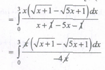
= \(-\cfrac { 1 }{ 4 } \int _{ 0 }^{ 3 }{ \left( \sqrt { x+1 } -\sqrt { 5x+1 } \right) dx } \)
= \(-\cfrac { 1 }{ 4 } \left[ \cfrac { \left( x+1 \right) ^{ \cfrac { 3 }{ 2 } } }{ \cfrac { 3 }{ 2 } } -\cfrac { \left( 5x+1 \right) ^{ \cfrac { 3 }{ 2 } } }{ 5\left( \cfrac { 3 }{ 2 } \right) } \right] _{ 0 }^{ 3 }\)
= \(-\cfrac { 1 }{ 4 } \left[ \cfrac { 2 }{ 3 } \left( x+1 \right) ^{ \frac { 3 }{ 2 } }-\cfrac { 1 }{ 15 } \left( 5x+1 \right) ^{ \frac { 3 }{ 2 } } \right] _{ 0 }^{ 3 }\)
= \(-\cfrac { 1 }{ 2 } \left[ \cfrac { 1 }{ 3 } \left( x+1 \right) ^{ \cfrac { 3 }{ 2 } }-\cfrac { 1 }{ 15 } \left( 5x+1 \right) ^{ \cfrac { 3 }{ 2 } } \right] _{ 0 }^{ 3 }\)
= \(-\cfrac { 1 }{ 2 } \left[ \cfrac { 1 }{ 3 } (4)^{ \cfrac { 3 }{ 2 } }-\cfrac { 1 }{ 15 } \left( 16 \right) ^{ \cfrac { 3 }{ 2 } } \right] -\left[ \cfrac { 1 }{ 3 } \left( 1 \right) ^{ \cfrac { 3 }{ 2 } }-\cfrac { 1 }{ 15 } \left( 1 \right) ^{ \cfrac { 3 }{ 2 } } \right] \)
= \(-\cfrac { 1 }{ 2 } \left[ \left( \cfrac { 1 }{ 3 } \left( 4 \right) \sqrt { 4 } -\cfrac { 1 }{ 15 } 16\sqrt { 16 } \right) -\left( \cfrac { 1 }{ 3 } -\cfrac { 1 }{ 15 } \right) \right] \)
= \(\cfrac { 1 }{ 2 } \left[ \left( \cfrac { 8 }{ 3 } -\cfrac { 64 }{ 15 } \right) -\cfrac { 1 }{ 3 } +\cfrac { 1 }{ 5 } \right] \)
= \(-\cfrac { 1 }{ 2 } \left[ \cfrac { 8 }{ 3 } -\cfrac { 64 }{ 15 } -\cfrac { 1 }{ 3 } +\cfrac { 1 }{ 15 } \right] \)
= \(-\cfrac { 1 }{ 2 } \left[ \cfrac { 8 }{ 3 } -\cfrac { 1 }{ 3 } -\cfrac { 64 }{ 15 } +\cfrac { 1 }{ 15 } \right] \)
= \(-\cfrac { 1 }{ 2 } \left[ \cfrac { 7 }{ 3 } -\cfrac { 63 }{ 15 } \right] =-\cfrac { 1 }{ 2 } \left[ \cfrac { 105-189 }{ 45 } \right] \)
= \(-\cfrac { 1 }{ 2 } \left[ \cfrac { -84 }{ 45 } \right] =\cfrac { 42 }{ 45 } =\cfrac { 14 }{ 15 } \)
\(\therefore\) \(I=\cfrac { 14 }{ 15 } \)
25.
In simple random sampling the samples are selected in such a way that each and every unit in the population has an equal and independent chance of being selected as a sample. It can be done with or without replacement of the samples selected. If the sampling is With replacement, there is a possibility of selecting the same sample any number of times. So, in simple random sampling without replacement is followed. Thus in simple random sampling from a population of N units, the probability is 1/ N the probability of drawing any unit in the second draw from among the available (N - 1) units is 1/(N - 1) and so on.
Simple random sampling without replacement is followed. The following two methods are generally used.
(A) Lottery method:
This is the most popular and simplest method when the population is finite. In this method, all the items of the population are numbered on separate slips of paper of same size, shape and colour. They are folded and placed in a container and shuffled thoroughly. Then the required numbers of slips are selected.
(B) Table of Random number:
The random number table has been so constructed that each of the digits 0,1,2, ... ,9 will appear approximately with the same frequency and independently of each other.
The various random number tables available are
a. L.H.C. Tippet random number series
b. Fisher and Yates random number series
c. Kendall and Smith random number series
d. Rand Corporation random number series.
Example: Tippett's table of random numbers is 20 items out of 6000.
Here we consider row wise selection of random numbers.
| 6641 | 9792 | 7969 | |||||
| 4167 | 9524 | 7203 | |||||
| 2670 | 7483 | 1089 | 6913 | 7991 | |||
| 6107 | 6008 | 8125 | 8776 | ||||
| 2754 | 9143 | 1405 | 9025 | 7002 | 6111 | 8816 | 6446 |
26.
\(\int _{ a }^{ b }{ f\left( x \right) } dx=\lim _{ x\rightarrow \infty \\ h\rightarrow 0 }{ \sum _{ r=1 }^{ n }{ h\ f(a+rh) } } \)
Here a = 0, b = 0
and f(x) = x + 4
f (a + rh) = \(f\left( 0+\frac { r }{ n } \right) =f\left( \frac { r }{ n } \right) \)
\(=\frac { r }{ n } +4\)
\(\therefore \int _{ 0 }^{ 1 }{ \left( x+4 \right) } dx=\lim _{ n\rightarrow \infty }{ \sum _{ r=1 }^{ n }{ \frac { 1 }{ n } } } \left( \frac { r }{ n } +4 \right) \)
\(=\lim _{ n\rightarrow \infty }{ \sum _{ r=1 }^{ n }{ \left( \frac { r }{ { n }^{ 2 } } +\frac { 4 }{ n } \right) } } \)
\(=\lim _{ n\rightarrow \infty }{ \left( \frac { 1 }{ { n }^{ 2 } } \sum _{ r=1 }^{ n }{ r } +\frac { 4 }{ n } \sum _{ r=1 }^{ n }{ 1 } \right) } \)
.JPG)
\(\left( \sum _{ r=1 }^{ n }{ 1=n)\sum _{ r=1 }^{ n }{ r } =\frac { n(n+2) }{ 2 } } \right) \)
.JPG)
\(=\lim _{ n\rightarrow \infty }{ \frac { 1+\frac { 1 }{ n } }{ 2 } } +4\)
\(=\frac { 1+0 }{ 2 } 4\)
[∵ when \(n\rightarrow \infty ,\frac { 1 }{ n } \rightarrow 0\)]
\(=\frac { 1 }{ 2 } +4=\frac { 1+8 }{ 2 } =\frac { 9 }{ 2 } \)
27.
Sample size n = 50 Sample mean \(\bar x\) = 10 km sample standard deviation s = 3.5 km
Population mean \(\mu\) = 9.5km
Since population SD is unknown we consider \(\sigma\) = s
The sample is a large sample and so we apply Z-test
Null Hypothesis :
There is no significant difference between the sample average and the company’s claim, i.e., \(H_0 : \mu=9.5\)
Alternative Hypothesis :
There is significant difference between the sample average and the company’s claim, i.e., H1 : \(\mu\)\(\neq \) 9.5 (two tailed test)
The level of significance \(\alpha\) = 5% = 0.05
Applying the test statistic
\(Z=\frac { \bar { x } -\mu }{ \frac { \sigma }{ \sqrt { n } } } \sim N(0,1);\ \)
\(Z=\frac { 10-9.5 }{ \frac { 3.5 }{ \sqrt { 50 } } } \sim N(0,1)=\frac { 0.5 }{ 0.495 } =1.01\)
Thus the calculated value 1.01 and the significant value or table value \({ Z }_{ \frac { \sigma }{ 2 } }=1.96\)
Comparing the calculated and table value ,Here Z<\({ Z }_{ \frac { \sigma }{ 2 } }\)i.e., 1.01<1.96.
Inference : Since the calculated value is less than table value i.e., Z < \({ Z }_{ \frac { \sigma }{ 2 } }\) at 5% level of sinificance, the null hypothesis H0 is accepted. Hence we conclude that the company’s claim that the new car petrol consumption is 9.5 km per litre is acceptable.
28.
Let I = \(\int _{ 2 }^{ 5 }{ \frac { \sqrt { x } }{ \sqrt { x } +\sqrt { 7-x } } } \) dx ...(1)
I = \(\int _{ 2 }^{ 5 }{ \frac { \sqrt { 2+5-x } }{ \sqrt { 2+5-x } +\sqrt { 7-(2+5-x) } } } \) dx \(\left[∵ \int _{ 0 }^{ a }{ f(x) } dx=\int _{ 0 }^{ a }{ f(a+b-x)dx } \right] \)
I = \(\int _{ 2 }^{ 5 }{ \frac { \sqrt { 7-x } }{ \sqrt { 7-x } +\sqrt { x } } } \)dx ..... (2)
(1) + (2) ⇒
2I = \(\int _{ 2 }^{ 5 }{ \left[ \frac { \sqrt { x } }{ \sqrt { x } +\sqrt { 7-x } } +\frac { \sqrt { 7+x } }{ \sqrt { 7-x } +\sqrt { x } } \right] } \) dx
= \(\int _{ 2 }^{ 5 }{ \left[ \frac { \sqrt { x } +\sqrt { 7-x } }{ \sqrt { x } +\sqrt { 7-x } } \right] } \) dx
= \(\int _{ 2 }^{ 5 }{ dx } \) = \({ \left[ x \right] }_{ 2 }^{ 5 }\) = 3
ஃ I = \(\frac { 3 }{ 2 } \)
29.
The first thing is to number the population (8585 children). The numbering has already been provided by the frequency table. There are 2 children with height of 105 cm, therefore we assign number 1 and 2 to the children those in the group 105 cm, number 3 to 6 is assigned to those in the group 107 cm and similarly all other children are assigned the numbers. In the last group 145 cms there are two children with assigned number 8584 and 8585.
| Height (cm) | Number of children | Cumulative Frequency |
| 105 | 2 | 2 |
| 107 | 4 | 6 |
| 109 | 14 | 20 |
| 111 | 41 | 61 |
| 113 | 83 | 144 |
| 115 | 169 | 313 |
| 117 | 394 | 707 |
| 119 | 669 | 1376 |
| 121 | 990 | 2366 |
| 123 | 1223 | 3589 |
| 125 | 1329 | 4918 |
| 127 | 1230 | 6148 |
| 129 | 1063 | 7211 |
| 131 | 646 | 7857 |
| 133 | 392 | 8249 |
| 135 | 202 | 8451 |
| 137 | 79 | 8530 |
| 139 | 32 | 8562 |
| 141 | 16 | 8578 |
| 143 | 5 | 8583 |
| 145 | 2 | 8585 |
| Total | 8585 |
Now we take 10 samples from the tables, since the population size is in 4 digits we can use the given random number table. Select the10 random numbers from 1 to 8585 in the table, Here, we consider column wise selection of random numbers, starting from first column.
| Tippet’s random number table | |||||||
| 2952 | 6641 | 3992 | 9792 | 7969 | 5911 | 3170 | 5624 |
| 4167 | 9524 | 1545 | 1396 | 7203 | 5356 | 1300 | 2693 |
| 2670 | 7483 | 3408 | 2762 | 3563 | 1089 | 6913 | 7991 |
| 0560 | 5246 | 1112 | 6107 | 6008 | 8125 | 4233 | 8776 |
| 2754 | 9143 | 1405 | 9025 | 7002 | 6111 | 8816 | 6446 |
The children with assigned number 2952 is selected and then see the cumulative frequency table where 2952 is present, now select the corresponding row height which is 123 cm, similarly all the selected random numbers are considered for the selection of the child with their corresponding height. The following table shows all the selected 10 children with their heights.
| Child with assigned Number | 2952 | 4167 | 2670 | 0560 | 2754 |
| Corresponding Height (cms) | 123 | 125 | 123 | 117 | 123 |
| Child with assigned Number | 6641 | 7483 | 5246 | 3996 | 1545 |
| Corresponding Height (cms) | 129 | 131 | 127 | 125 | 121 |
30.
Given μ = 400, σ = 100
(i) Company pays a penalty of atleast Rs. 2,00,000
Penalty per day = Rs.10,000
Number of days = \(\frac { 2,00,000 }{ 10,000 } \) = 20
Hence, the company has taken excess of 20 days
∴ P(atleast 470 days) [∵ 450 + 20 = 470]
= P(X ≥ 470)
When X = 470, Z = \(\frac { X-\mu }{ \sigma } \)
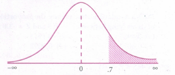
= \(\frac { 470-400 }{ 100 } =\frac { 70 }{ 100 } \) = 0.7
∴ P(X ≥ 470) = P(Z ≥ 0.7)
= P(0.7
P(X ≥ 470) = 0.2420
(ii) P (atmost 500 days) = P(X≤500)
When X = 500, Z = \(\frac { X-\mu }{ \sigma } \)
= \(\frac { 500-400 }{ 100 } =\frac { 100 }{ 100 } \)=1
∴ P(X ≤ 500) = P(Z≤1)
= P(-∞
= 0.8413
P(X ≤ 500) = 0.8413
31.
Plot the variable X = 50 on the left side and
X = 86 on the right side of the curve.
Given P( -∞< Z1 < -Z1) = 0.3
⇒ P(-Z1 < Z < Z1) = 0.2 [∵ 0.5 - 0.3 = 0.2]
⇒ P(0 < Z < Z1) = 0.2 [By symmetry]
⇒ Z1 = -0.52 [From the normal distribution table 'and it lies on the negative side]
⇒ -0.52 = \(\frac { X-\mu }{ \sigma } \) ⇒ -0.52 σ = 50-μ
⇒ 50-μ = -0.52 σ ....(1)
Also given P(Z2
⇒ Z2 = 1.28 (from the table)
⇒ 1.28 =\(\frac { 86-\mu }{ \sigma } \)
⇒ 86-μ = 1.28 σ ...(2)
Substituting σ = 20 in (2) we get,
86-μ = (1.28)(20)
86-μ = 25.6
μ = 86-25.6
μ = 60.4
Hence, the mean is 60.4 and standard deviation is 20.
32.
Given mean = λ = 1.5
X follows poisson distribution with
p(x,λ) = \(\frac { e^{ -\lambda }.{ \lambda }^{ x } }{ x! } \)
(i) ∴ P(neither car is used)
= P(X = 0) = \(\frac { e^{ -1.5 }.(1.5)^{ 0 } }{ 0! } \) =e-1.5
= 0.2231 [∵ e-1.5 =0.2231]
(ii) P (Some demand is refused)
The demand may be either 0 car, 1 car or 2 cars
∴ P (Some demand is refused) = 1 - P(X ≤ 2)
= 1 - [P(X = 0) + P (X = 1) + P(X = 2)]
= 1-\(\left[ \frac { e^{ -\lambda }.{ \lambda }^{ 0 } }{ 0! } +\frac { e^{ -\lambda }.{ \lambda }^{ 1 } }{ 1! } +\frac { e^{ -\lambda }.{ \lambda }^{ 2 } }{ 2! } \right] \)
= 1-e-λ (1+λ+\(\frac { { \lambda }^{ 2 } }{ 2 } \))
= 1-e-1.5 (1+1.5+\(\frac { (1.5)^{ 2 } }{ 2 } \))
= 1 - 0.2231 (3.625) = 1 - 0.8087 = 0.1912
∴ Probability of some demand is refused = 0.1912.
33.
34.
Let X be the waiting time of a customer in the queue and it is normally distributed with mean 5 and SD 0.7.
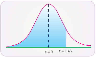
(i) for less than 6 minutes
\(Z=\frac { X-\mu }{ \sigma } =\frac { 6-5 }{ 0.7 } =1.4285\)
P(X < 6) = P(Z < 1.43)
= 0.5 + 0.4236
= 0.9236
(ii) between 3.5 and 6.5 minutes
When X = 3.5
\(Z=\frac { X-\mu }{ \sigma } =\frac { 3.5-5 }{ 0.7 } =2.1429\)
When X = 6.5
\(Z=\frac { X-\mu }{ \sigma } =\frac { 6.5-5 }{ 0.7 } =2.1429\)
P(3.5 < X < 6.5)
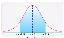
= P (–2.1429 < Z < 2.1429)
= P(0 < Z < 2.1429) + P(0 < Z < 2.1429)
= 2 P(0 < Z < 2.1429)
= 2 x .4838
= 0.9676
35.
Here mean μ= 30 and standard deviation σ = 5
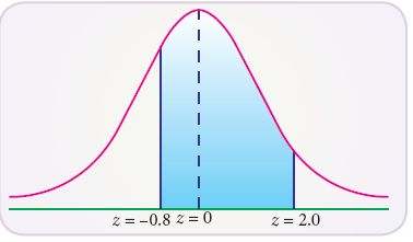
(i) When X = 26 Z=(X−μ)/\(\sigma \) = (26 – 30)/5 = –0.8
And when X = 40 , z =\(\frac{40-30}{5}=2\)
Therefore,
P(26 < x < 40))
= P(–0.8 ≤ Z ≤ 0) + p(0 ≤ Z ≤ 2)
= P(0 ≤ Z ≤ 0.8) + P(0 ≤ Z ≤ 2)
= 0.2881 + 0.4772 (By tables)
= 0.7653
(ii) The probability that X≥45
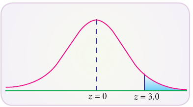
When X = 45
\(z=\frac { X-\mu }{ \sigma } =\frac { 45-30 }{ 5 } =3\)
P( X ≥ 45) = P(Z ≥ 3)
= 0.5 – 0.49865
= 0.00135
36.
Probability of raining on a particular day is given by p = 9/30 = 3/10 and q = 1–p = 7/10.
The binomial distribution is P(X = x) = nCx px qn–x
There are 7 days in a week
P(X = x) =\(\left( \begin{matrix} 7 \\ x \end{matrix} \right) { \left( \frac { 3 }{ 10 } \right) }^{ x }{ \left( \frac { 7 }{ 10 } \right) }^{ 7-x }\)
The probability of raining for atleast 2 days is given by
P(X\(\ge\)2) = 1-P(X<2)
= 1-[P(X = 0)+P(X = 1)]
Here, P(X = 0)\(\left( \begin{matrix} 7 \\ 0 \end{matrix} \right) { \left( \frac { 3 }{ 10 } \right) }^{ 0 }{ \left( \frac { 7 }{ 10 } \right) }^{ 7-0 }\)
= 0.0823
and \(P(X=1)=\left( \begin{matrix} 7 \\ 1 \end{matrix} \right) \left( \frac { 3 }{ 10 } \right) { \left( \frac { 7 }{ 10 } \right) }^{ 7-1 }\)
= 0.2471
Therefore the required probability = 1– [P(x = 0) +P(x = 1)]
= 1– [0.082+ 0.247]
= 0.6706
37.
Given p.d.f is = \(f(x)=\left\{\begin{array}{l} a+b x^{2}, 0 \leq x \leq 1 \\ 0, \text { otherwise } \end{array}\right.\)
Since f(x) is a p.d.f.\(\\ \int _{ -\infty }^{ \infty }{ f(x)dx=1 } \)
\(\Rightarrow \int _{ 0 }^{ 1 }{ (a+{ bx }^{ 2 })dx=1 } \)
\(\Rightarrow { \left[ ax+\frac { { bx }^{ 3 } }{ 3 } \right] }_{ 0 }^{ 1 }=1\Rightarrow a+\frac { b }{ 3 } =1\)
3a+b = 3 [multiplied by 3] ...(1)
Also it is given that E(X) = \(\frac{3}{5}\)
\(\Rightarrow \int _{ 0 }^{ 1 }{ x.f(x)dx=\frac { 3 }{ 5 } } \)
\(\Rightarrow \int _{ 0 }^{ 1 }{ (a+{ bx }^{ 2 })dx=\frac { 3 }{ 5 } } \)
\(\Rightarrow \int _{ 0 }^{ 1 }{ (ax+{ bx }^{ 3 })dx=\frac { 3 }{ 5 } } \)
\(\Rightarrow { \left[ \frac { { ax }^{ 2 } }{ 2 } +\frac { { bx }^{ 4 } }{ 4 } \right] }_{ 0 }^{ 1 }=\frac { 3 }{ 5 } \Rightarrow \frac { a }{ 2 } +\frac { b }{ 4 } =\frac { 3 }{ 5 } \)
\(\Rightarrow 2a+b=\frac { 12 }{ 5 } \) [Multiplies by 4] ...(2)
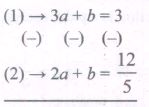
\(a=3-\frac { 12 }{ 5 } =\frac { 15-12 }{ 5 } =\frac { 3 }{ 5 } \)
Substituting a=\(\frac{3}{5}\) in(2) we get,
\(2(\frac { 3 }{ 5 } )+b=\frac { 12 }{ 5 } \Rightarrow \frac { 6 }{ 5 } +b=\frac { 12 }{ 5 } \)
\(\Rightarrow b=\frac { 12 }{ 5 } -\frac { 6 }{ 5 } =\frac { 6 }{ 5 } \)
\(\therefore a=\frac { 3 }{ 5 } ,b=\frac { 6 }{ 5 } \)
ii) \(E({ X }^{ 2 })=\int _{ 0 }^{ 1 }{ { x }^{ 2 }f(x)dx=\int _{ 0 }^{ 1 }{ { x }^{ 2 }\left( \frac { 3 }{ 5 } +\frac { 6 }{ 5 } { x }^{ 2 } \right) dx } } \)
\(\left[ \because a=\frac { 3 }{ 5 } ,b=\frac { 6 }{ 5 } \right] \)
\(=\int _{ 0 }^{ 1 }{ \left( \frac { 3 }{ 5 } { x }^{ 2 }+\frac { 6 }{ 5 } { x }^{ 4 } \right) dx } \)
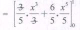
\(=\frac { 1 }{ 5 } (1-0)+\frac { 6 }{ 25 } (1-0)\)
\(=\frac { 1 }{ 5 } +\frac { 6 }{ 25 } =\frac { 5+6 }{ 25 } =\frac { 11 }{ 25 } \)
\(\therefore\) Var (X) = E(X2)-[E(X)]2
\(=\frac { 11 }{ 25 } -{ \left( \frac { 3 }{ 5 } \right) }^{ 2 }\)
\(=\frac { 11 }{ 25 } -\frac { 9 }{ 25 } =\frac { 2 }{ 25 } \)
\(\therefore\) Var (X) =\(\frac{2}{25}\)
38.
Let I = ∫ ex(1+x) log(xex)dx
Put t = x ex
⇒ dt = (x.ex + ex(1))dx
= ex(x+1)dx
∴ I = ∫ log t.dt
Let u = log t; dv = dt
\(du=\frac { 1 }{ t } dt;v=t\)
∴Using integration by parts we get,
I = ∫udv = vu - ∫vdu
= t log t - ∫dt = t logt - t + c
= t log t - t + c
= xex log(xex) - (xex) + c [∵ t = xex]
= xex (log(xex)-1)+c
39.
Given demand function Pd = 20 - 5x and
Supply function Ps = 4x + 8
Under market equilibrium ps = Pd
⇒ 20-5x = 4x+8
⇒ 20-8 = 4x+5x
⇒ 12 = 9x
\(\Rightarrow x=\frac{\not 12}{\not 9}=\frac{4}{3}\)
When \({ x }_{ 0 }=\frac { 4 }{ 3 } ,{ p }_{ 0 }=20-5\left( \frac { 4 }{ 3 } \right) =20-\frac { 20 }{ 3 } \)
\(=\frac { 60-20 }{ 3 } =\frac { 40 }{ 3 } \)
\(\therefore { p }_{ 0 }{ x }_{ 0 }=\frac { 40 }{ 3 } \times \frac { 4 }{ 3 } =\frac { 160 }{ 9 } \)
Consumer Surplus (CS)
\(=\int _{ 0 }^{ x }{ f(x)dx } -{ p }_{ 0 }{ x }_{ 0 }\)
\(=\int _{ 0 }^{ \frac { 4 }{ 3 } }{ (20-5x)dx } \)
\(={ \left[ 20x-\frac { { 5x }^{ 2 } }{ 2 } \right] }_{ 0 }^{ \frac { 4 }{ 3 } }-\frac { 160 }{ 9 } \)
\(=20\left( \frac { 4 }{ 3 } \right) -\frac { 5 }{ 2 } \left( \frac { 16 }{ 9 } \right) -\frac { 160 }{ 9 } \)
\(=\frac { 80 }{ 3 } -\frac { 40 }{ 9 } -\frac { 160 }{ 9 } \)
\(=\frac { 240-40-160 }{ 9 } =\frac { 40 }{ 9 } \)
\(\therefore CS=\frac { 40 }{ 9 }\)units
Producer's Surplus
\((PS)={ p }_{ 0 }{ x }_{ 0 }-\int _{ 0 }^{ x }{ g(x)dx } \)
\(=\frac { 160 }{ 9 } -\int _{ 0 }^{ \frac { 4 }{ 3 } }{ (4x+8)dx } \)
\(=\frac { 160 }{ 9 } -{ \left[ \frac { { 4x }^{ 2 } }{ 2 } +8x \right] }_{ 0 }^{ \frac { 4 }{ 3 } }\)
\(=\frac { 160 }{ 9 } -\left( 2\left( \frac { 16 }{ 9 } \right) +8\left( \frac { 4 }{ 3 } \right) \right) \)
\(=\frac { 160 }{ 9 } -\left( \frac { 32 }{ 9 } +\frac { 32 }{ 3 } \right) \)
\(=\frac { 160 }{ 9 } -\frac { 32 }{ 9 } -\frac { 32 }{ 3 } \)
\(PS=\frac { 160-32-96 }{ 9 } =\frac { 32 }{ 9 } \)units
40.
Mean of the random variableX = E(X) = \({ \sum_x { x{ P }_{ x }(x) } } \)
= (1 × 0.15) + (2 × 0.10) + (3 × 0.10) + (4 × 0.01) + (5 × 0.08) + (6 × 0.01) +(7 × 0.05) + (8 × 0.02) + (9 × 0.28) + (10 × 0.20)
E(X) = 6.18
E(X2) = \(\sum _{ x }^{ }{ { x }^{ 2 } } { P }_{ X }(x)\)
= (12 × 0.15) + (22 × 0.10) + (32 × 0.10) + (42 × 0.01) + (52 × 0.08) + (62 × 0.01) + (72 × 0.05) + (82 × 0.02) + (92 × 0.28) + (102 × 0.20).
= 50.38
Variance of the Random Variagble X = V(X) = E(X2)-[E(X)]2
=50.38-(6.56)2
= 12.19
Therefore, the mean and variance of the given discrete distribution are 6.18 and 12.19 respectively.
41.
Given C'(x) = 5 + 0.13x
R'(x) = 18
Fixed cost is Rs. 120
C'(x) = 5 + 0.13x
⇒ ∫C'(x) = ∫(5+0.13x)dx
⇒ C(x) = 5x \(+\frac { 0.13{ x }^{ 2 } }{ 2 } +{ k }_{ 1 }\)
Since fixed cost is Rs.120 ⇒ k1 = 120
\(\therefore C(x)=5x+\frac { 0.13{ x }^{ 2 } }{ 2 } +120\) ...(1)
Also R'(x) = 18
⇒ ∫R'(x) = ∫18dx
⇒ R(x) = 18x+k2
When x = 0, R = 0 ⇒ k2= 0
∴ R(x) = 18x ...(2)
Profit function ⇒ P(x) = R(x) - C(x)
\(=18x-5x-\frac { 0.13{ x }^{ 2 } }{ 2 } -120\)
[from (1) & (2)]
P(x) = 13x-0.065x2-120
42.
Given p.d.f is
\(f(x)=\begin{cases} \begin{matrix} \frac { 1 }{ 16 } { (3+x) }^{ 2 }, & -3\le x\le -1 \end{matrix} \\ \begin{matrix} \frac { 1 }{ 16 } (6-2{ x }^{ 2 }), & -1\le x\le 1 \end{matrix} \\ \begin{matrix} \frac { 1 }{ 16 } { (3-x) }^{ 2 }, & 1\le x\le 3 \end{matrix} \end{cases}\)
Area under the given curve
\(\int _{ -3 }^{ 3 }{ f(c)dx=\int _{ -3 }^{ -1 }{ \frac { 1 }{ 16 } { (3+x) }^{ 2 }+\int _{ -1 }^{ 1 }{ \frac { 1 }{ 16 } (6-2{ x }^{ 2 })dx } } +\int _{ 1 }^{ 3 }{ \frac { 1 }{ 16 } { (3-x) }^{ 2 }dx } } \)
\(=\frac { 1 }{ 16 } { \left[ \frac { (3+x{ ) }^{ 3 } }{ 3 } \right] }_{ -3 }^{ -1 }+\frac { 1 }{ 16 } { \left( 6x-\frac { { 2x }^{ 3 } }{ 3 } \right) }_{ -1 }^{ 1 }+\frac { 1 }{ 16 } { \left( \frac { { (3-x) }^{ 3 } }{ -3 } \right) }_{ 1 }^{ 3 }\)
\(=\frac { 1 }{ 16 } \left[ \left( \frac { { 2 }^{ 3 } }{ 3 } -0 \right) +\left( 6-\frac { 2 }{ 3 } \right) -\left( -6+\frac { 2 }{ 3 } \right) -\frac { 1 }{ 3 } \left( 0-({ 2 }^{ 3 }) \right) \right] \)
\(=\frac { 1 }{ 6 } \left[ \frac { 8 }{ 3 } +\frac { 16 }{ 3 } -\left( \frac { -16 }{ 3 } \right) +\frac { 8 }{ 3 } \right] \)
\(\\ =\frac { 1 }{ 16 } \left[ \frac { 8 }{ 3 } +\frac { 16 }{ 3 } +\frac { 16 }{ 3 } +\frac { 8 }{ 3 } \right] \)
\(=\frac { 1 }{ 16 } \left[ \frac { 8+16+16+8 }{ 3 } \right] \)
\(=\frac { 1 }{ 16 } \times \frac { 48 }{ 3 } =\frac { 1 }{ 16 } \times 16=1\)
Hence, area under the given curve is unity.
43.
\(\frac { { E }_{ y } }{ { E }_{ x } } =\frac { x }{ x-2 } \)
\(\frac { { xd }_{ y } }{ { yd }_{ x } } =\frac { x }{ x-2 } \)
\(\frac { dy }{ y } =\frac { x }{ x-2 } .\frac { dx }{ x } \)
\(\int { \frac { dy }{ y } } =\int { \frac { dx }{ x-2 } } \)
log y = log(x − 2) + log k
y = k(x–2)
when x = 6, y = 16 ⇒ 16 = k(6–2)
k = 4
y = 4 (x–2)
44.
Given C(x) = \(\int { C' } (x)dx+\)k1
= \(\int { \left( 50+\frac { x }{ 50 } \right) } \)dx +k1
C(x) = 50x + \(\frac{x^2}{100}\)+k1
When quantity produced is zero, then the fixed cost is 200.
i.e. When x = 0, c = 200
⇒ k1 = 200
Cost function is C(x) = 50x + \(\frac{x^2}{100}\) + 200 (1)
The Revenue R'(x) = 60
R(x) = \(\int { R' } (x)dx\) + k2
\(\int { 60 } dx\)+ k2
= 60x + k2
When no product is sold, revenue = 0
i.e. When x = 0, R = 0
Revenue R(x) = 60x (2)
Profit P = Total Revenue – Total cost
= 60x - 50x - \(\frac { { x }^{ 2 } }{ 100 } \) - 200
= 10x - \(\frac { { x }^{ 2 } }{ 100 } \) - 200
\(\frac { dp }{ dx } =10-\frac { x }{ 50 } \)
To get profit maximum, \(\frac { dp }{ dx } \) = 0 ⇒ x = 500
\(\frac { { d }^{ 2 }P }{ { dx }^{ 2 } } =\frac { -1 }{ 50 } <0\)
ஃ Profit is maximum when x = 500 and
Maximum Profit is P = 10(500) - \(\frac { { (500) }^{ 2 } }{ 100 } \) - 200
= 5000 – 2500 – 200
= 2300
Profit = Rs. 2,300.
45.
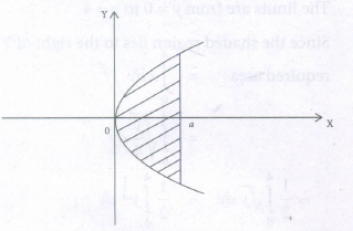
46.
\(\int { \frac { { 4x }^{ 2 }+2x+6 }{ { \left( x+1 \right) }^{ 2 }-(x-3) } } dx\)
\(=\int { \left( \frac { A }{ x+1 } +\frac { B }{ { \left( x+1 \right) }^{ 2 } } +\frac { C }{ x-3 } \right) } dx\)
\(=\left( \frac { 1 }{ x+1 } +\frac { -2 }{ { \left( x+1 \right) }^{ 2 } } +\frac { 3 }{ x-3 } \right) dx\)
4x2+2x+6 = A (x+1) (x-3) + B(x-3) + (x+1)2
⇒ Putting x = -1, 4-2+6 = B(-4)
⇒ 8 = B(-4) ⇒ B = -2
Putting x = 3
36 + 6 + 6 = C (16)
⇒ 48 = 16C
⇒ C = 3
Putting x = 0,
6 = -3A -3B + C
⇒ 6 = -3A + 6 + 3
⇒ 3A = 3
⇒ A = 1
\(=\log { \left| x+1 \right| } -2\int { { \left( x+1 \right) }^{ -2 } } dx+3\log { \left| x-3 \right| } +c\)
\(=\log { \left| x+1 \right| } -2\frac { { \left( x+1 \right) }^{ -2+1 } }{ -2+1 } +3\log { \left| x-3 \right| } +c\)
\(=\log { \left| x+1 \right| } +2{ \left( x+1 \right) }^{ -1 }+3\log { \left| x-3 \right| } +c\)
\(=\log { \left| x+1 \right| } +\frac { 2 }{ x+1 } +3\log { \left| x-3 \right| } +c\)
47.
\(\Delta =\left| \begin{matrix} 1 & 2 & 1 \\ 2 & -1 & 2 \\ 1 & 1 & -2 \end{matrix} \right| \)
= \(1\left| \begin{matrix} -1 & 2 \\ 1 & -2 \end{matrix} \right| -2\left| \begin{matrix} 2 & 2 \\ 1 & -2 \end{matrix} \right| +1\left| \begin{matrix} 2 & -1 \\ 1 & 1 \end{matrix} \right| \)
= 1(2 -2) - 2(-4 -2) + 1(2 + 1)
= 1(0)-2(-6)+1(3)
= 12 + 3 = 15\(\neq \)0.
Since \(\Delta \neq 0\) Cramer's rule can be applied and thesystem is consistent with unique solution.
\({ \Delta }x=\left| \begin{matrix} 7 & 2 & 1 \\ 4 & -1 & 2 \\ -1 & 1 & -2 \end{matrix} \right| \)
= \(7\left| \begin{matrix} -1 & 2 \\ 1 & -2 \end{matrix} \right| -2\left| \begin{matrix} 4 & 2 \\ -1 & -2 \end{matrix} \right| +1\left| \begin{matrix} 4 & -1 \\ -1 & 1 \end{matrix} \right| \)
= 7 (2 -2) -2 (-8 + 2) + 1 (4 - 1)
= 7 (0) - 2(-6) + 1(3)
= 12 + 3 = 15
\(\Delta y=\left| \begin{matrix} 1 & 7 & 1 \\ 2 & 4 & 2 \\ 1 & -1 & -2 \end{matrix} \right| \)
= \(1\left| \begin{matrix} 4 & 2 \\ -1 & -2 \end{matrix} \right| -7\left| \begin{matrix} 2 & 2 \\ 1 & -2 \end{matrix} \right| +1\left| \begin{matrix} 2 & 4 \\ 1 & -1 \end{matrix} \right| \)
= 1 (- 8 + 2) -7(-4 -2) + 1(-2 -4)
= 1 (-6) -7 (-6) + 1 (-6)
= - 6 + 42 - 6 = 30
\(\Delta z=\left| \begin{matrix} 1 & 2 & 7 \\ 2 & -1 & 4 \\ 1 & 1 & -1 \end{matrix} \right| \)
= \(1\left| \begin{matrix} -1 & 4 \\ 1 & -1 \end{matrix} \right| -2\left| \begin{matrix} 2 & 4 \\ 1 & -1 \end{matrix} \right| +7\left| \begin{matrix} 2 & -1 \\ 1 & 1 \end{matrix} \right| \)
= 1 (1 - 4) - 2(- 2 - 4) + 7(2 + 1)
= 1(-3)-2(-6)+7(3)
= - 3 + 12 + 21 = 30
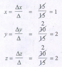
\(\therefore\) Solution set is {1, 2, 2}
48.
Transition probability matrix
(A B) T = (A B)
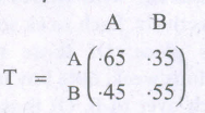
Where A represents the percent of people those who bought soap A and B represents the percent of people those who bought soap B.
By the given data
A = 15% = ·15
and B = 85% = ·85
Percentage after one year is
\(\left( \cdot 15\quad \cdot 85 \right) \left( \begin{matrix} \cdot 65 & \cdot 35 \\ \cdot 45 & \cdot 55 \end{matrix} \right) \)
= ((.15)(·65) + (·85)(-45) ·15(-35)+ ·85(-55))
= (-0975 + ·3825 ·0525 + -4675)
= (-48 ·52)
Hence, market share after one year is 48% and 52% At equilibrium,
\(\left( A\quad B \right) \left( \begin{matrix} \cdot 65 & \cdot 35 \\ \cdot 45 & \cdot 55 \end{matrix} \right) =(A\quad B)\)
(-65A + A5B ·35A +·55B) = (A B)
Equating the corresponding entries on both sides we get
\(\Rightarrow \cdot 65A+\cdot 45B=A\)
\(\Rightarrow \cdot 65A+\cdot 45(1-A)=A\)
[Since A+B = 1 B = 1-A]
\(\Rightarrow \cdot 65A+\cdot 45-\cdot 45A=A\)
\(\Rightarrow \cdot 45=A-\cdot 65A+\cdot 45A\)
\(\Rightarrow \cdot 45=A\left( \cdot 35+45 \right) \)
\(\Rightarrow \cdot 45=A(\cdot 35+45)\)
\(\Rightarrow \cdot 45=A(-8)\)
\(\Rightarrow A=\cfrac { \cdot 45 }{ \cdot 8 } =\cdot 5625=56.25\)
\(\therefore B=1-A=1-\cdot 5625=\cdot 4375\)
= 43.75%
\(\therefore\) Equilibrium is reached when A = 56.25% and B = 43.75%
49.
Let ‘x’ be the number of cars of type C1
Let ‘y’ be the number of cars of type C2
Let ‘z’ be the number of cars of type C3
3x + 2y + 4z = 28
x + y + 2z =13
2x + 2y + z =14
Here \({ \triangle }=\left| \begin{matrix} 3 & 2 & 4 \\ 1 & 1 & 2 \\ 2 & 2 & 1 \end{matrix} \right| =-3\neq 0\)
\({ \triangle }_{ x }=\left| \begin{matrix} 28 & 2 & 4 \\ 13 & 1 & 2 \\ 14 & 2 & 1 \end{matrix} \right| =-6\)
\({ \triangle }_{ y }=\left| \begin{matrix} 3 & 28 & 4 \\ 1 & 1 & 2 \\ 2 & 2 & 1 \end{matrix} \right| =-9\)
\({ \triangle }_{ z }=\left| \begin{matrix} 3 & 2 & 28 \\ 1 & 1 & 13 \\ 2 & 2 & 14 \end{matrix} \right| =-12\)
\(\therefore \) By Cramer’s rule
\(x=\frac { { \triangle }x }{ { \triangle } } =\frac { -6 }{ -3 } =2\)
\(y=\frac { { \triangle }y }{ { \triangle } } =\frac { -9 }{ -3 } =3\)
\(z=\frac { { \triangle }z }{ { \triangle } } =\frac { -12 }{ -3 } =4\)
\(\therefore \) The number of cars of each type which can be produced are 2, 3 and 4.
50.
Given that the price of commodities X, Y and Z are x, y and z respectively
By the given data
| Transaction | x | y | z | Earning |
|---|---|---|---|---|
| Mr. Anand | +2 | +3 | -6 | Rs.5000 |
| Mr. Amar | +3 | -1 | +2 | Rs.2000 |
| Mr. Amit | -1 | +3 | +1 | Rs.5500 |
Here, purchasing is taken as negative symbol and selling is taken as positive symbol
Thus, the non-homogeneous equations are
2x + 3y - 6z = 5000
3x - y + 2z = 2000
-x + 3y + z = 550
The matrix equation corresponding to the given system is
\(\left( \begin{matrix} 2 & 3 & -6 \\ 3 & -1 & 2 \\ -1 & 3 & 1 \end{matrix} \right) \left( \begin{matrix} x \\ y \\ z \end{matrix} \right) =\left( \begin{matrix} 5000 \\ 2000 \\ 5500 \end{matrix} \right) \)
| Augmented matrix | Elementary Transformation |
|---|---|
| \(\left( \begin{matrix} 2 & 3 & -6 \\ 3 & -1 & 2 \\ -1 & 3 & 1 \end{matrix}\begin{matrix} 5000 \\ 2000 \\ 5500 \end{matrix} \right) \) | |
| \(\left( \begin{matrix} -1 & 3 & 1 \\ 3 & -1 & 2 \\ 2 & 3 & -6 \end{matrix}\begin{matrix} 5500 \\ 2000 \\ 5000 \end{matrix} \right) \) |  |
| \(\left( \begin{matrix} 1 & -3 & -1 \\ 3 & -1 & 2000 \\ 2 & 3 & -6 \end{matrix}\begin{matrix} -5000 \\ 2000 \\ 5500 \end{matrix} \right) \) | \({ R }_{ 1 }\rightarrow { R }_{ 1 }\left( -1 \right) \) |
| \(\left( \begin{matrix} 1 & -3 & -1 \\ 0 & 8 & 5 \\ 0 & 9 & -4 \end{matrix}\begin{matrix} -5500 \\ 18500 \\ 16000 \end{matrix} \right) \) | \({ R }_{ 2 }\rightarrow { R }_{ 2 }-3{ R }_{ 1 }\) \({ R }_{ 3 }\rightarrow { R }_{ 3 }-2{ R }_{ 1 }\) |
| \(\left( \begin{matrix} 1 & -3 & -1 \\ 0 & 1 & \frac { 65 }{ 8 } \\ 0 & 1 & \frac { -4 }{ 9 } \end{matrix}\begin{matrix} -5500 \\ \frac { 18500 }{ 8 } \\ \frac { 16000 }{ 9 } \end{matrix} \right) \) | \({ R }_{ 2 }\rightarrow { R }_{ 2 }\div 8\) \({ R }_{ 3 }\rightarrow { R }_{ 3 }\div 9\) |
| \(\left( \begin{matrix} 1 & -3 & -1 \\ 0 & 1 & \frac { 5 }{ 8 } \\ 0 & 0 & \frac { -4 }{ 9 } -\frac { 5 }{ 8 } \end{matrix}\begin{matrix} -5500 \\ \frac { 18500 }{ 8 } \\ \frac { 16000 }{ 9 } -\cfrac { 18500 }{ 8 } \end{matrix} \right) \) | \({ R }_{ 3 }\rightarrow R_{ 3 }-{ R }_{ 2 }\) |
| \(\left( \begin{matrix} 1 & -3 & -1 \\ 0 & 1 & \frac { 5 }{ 8 } \\ 0 & 0 & \frac { -77 }{ 72 } \end{matrix}\begin{matrix} -5500 \\ \frac { 18500 }{ 8 } \\ \frac { -38500 }{ 72 } \end{matrix} \right) \) |
.Clearly the last equivalent matrix is in echelon form and it has three non-zero rows
\(\therefore \rho (A)=\rho \left( \left[ A,B \right] \right) =3\) Number of unknowns.
\(\therefore\) The given system is consistent and has unique solution. To find the solution, let us rewrite the above : echelon form into the matrix form.
\(\left( \begin{matrix} 1 & -3 & -1 \\ 0 & 1 & \frac { 5 }{ 8 } \\ 0 & 0 & \frac { -77 }{ 72 } \end{matrix} \right) \left( \begin{matrix} x \\ y \\ z \end{matrix} \right) \left( \begin{matrix} -5000 \\ \frac { 18500 }{ 8 } \\ \frac { -38500 }{ 72 } \end{matrix} \right) \)
\(\Rightarrow x-3y-z=-5500\)
\(y+\cfrac { 5 }{ 8 } z=\cfrac { 18500 }{ 8 } \)
\(\cfrac { -77 }{ 72 } z=\cfrac { 38500 }{ 72 } \)
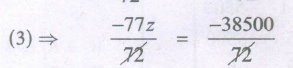
\(\Rightarrow z=\cfrac { -38500 }{ -77 } \)
\(\Rightarrow z=500\)
\((2)\Rightarrow y+\cfrac { 5 }{ 8 } \left( 500 \right) =\cfrac { 18500 }{ 8 } \)
\(y=\cfrac { 18500 }{ 8 } -\cfrac { 2500 }{ 8 } \)
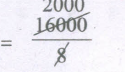
\(\Rightarrow y=2000\)
\((1)\Rightarrow x-3\left( 2000 \right) -500=-5500\)
\(\Rightarrow x-6000-500=-5500\)
\(\Rightarrow x-6000-500=-5500\)
\(\Rightarrow x=-5500+6500\)
\(\Rightarrow x=1000\)
Hence, the prices per unit of three commodities are Rs.1000, Rs. 2000 and Rs. 500 respectively
51.
The matrix equation corresponding to the given system is
\(\left( \begin{matrix} 1 & 1 & 1 \\ 1 & 2 & 3 \\ 1 & 2 & a \end{matrix} \right) \left( \begin{matrix} X \\ Y \\ Z \end{matrix} \right) =\left( \begin{matrix} 6 \\ 10 \\ b \end{matrix} \right) \)
AX = B
| Augmented matrix [A,B] | Elementary Transformation |
| \(\left( \begin{matrix} 1 & 1 & 1 \\ 1 & 2 & 3 \\ 1 & 2 & a \end{matrix}\begin{matrix} 6 \\ 10 \\ b \end{matrix} \right) \) \(\sim \left( \begin{matrix} 1 & 1 & 1 \\ 0 & 1 & 2 \\ 0 & 1 & a-1 \end{matrix}\begin{matrix} 6 \\ 4 \\ b-6 \end{matrix} \right) \) \(\sim \left( \begin{matrix} 1 & 1 & 1 \\ 0 & 1 & 2 \\ 0 & 0 & a-3 \end{matrix}\begin{matrix} 6 \\ 4 \\ b-10 \end{matrix} \right) \) |
\({ R }_{ 2 }\rightarrow { R }_{ 2 }-{ R }_{ 1 }\) \({ R }_{ 3 }\rightarrow { R }_{ 3 }-{ R }_{ 1 }\) |
Case (i) For no solution:
The system possesses no solution only when \(\rho (A)\neq ([A,B])\) which is possible only when a−3 = 0 and b −10 \(\neq \) 0.
Hence for a = 3, b \(\neq \) 10, the system possesses no solution.
Case (ii) For a unique solution:
The system possesses a unique solution only when \(\rho (A)= ([A,B])\)=number of unknowns.
i.e when \(\rho (A)=\rho ([A,B])\) = 3
Which is possible only when a−3 \(\neq \) 0 and b may be any real number as we can observe .
Hence for a \(\neq \) and b \(\in \) R, the system possesses a unique solution.
Case (iii) For an infinite number of solutions:
The system possesses an infinite number of solutions only when
\(\rho (A)=\rho ([A,B])\)
Hence for a = 3, b = 10, the system possesses infinite number of solutions.
52.
The matrix equation corresponding to the given system is
\(\left( \begin{matrix} 1 & 1 & 1 \\ 1 & 2 & 3 \\ 1 & 4 & 7 \end{matrix} \right) \left( \begin{matrix} X \\ Y \\ Z \end{matrix} \right) =\left( \begin{matrix} 6 \\ 14 \\ 30 \end{matrix} \right) \)
A X = B
| Augmented matrix [A,B] | Elementary Transformation |
| \(\left( \begin{matrix} 1 & 1 & 1 \\ 1 & 2 & 3 \\ 1 & 4 & 7 \end{matrix}\begin{matrix} 6 \\ 14 \\ 30 \end{matrix} \right) \) \(\sim \left( \begin{matrix} 1 & 1 & 1 \\ 0 & 1 & 2 \\ 0 & 2 & 4 \end{matrix}\begin{matrix} 6 \\ 8 \\ 16 \end{matrix} \right) \) \(\sim \left( \begin{matrix} 1 & 1 & 1 \\ 0 & 1 & 2 \\ 0 & 0 & 0 \end{matrix}\begin{matrix} 6 \\ 8 \\ 0 \end{matrix} \right) \) |
\({ R }_{ 2 }\rightarrow { R }_{ 2 }-{ R }_{ 1 }\) \({ R }_{ 3 }\rightarrow { R }_{ 3 }-{ R }_{ 2 }\) \({ R }_{ 3 }\rightarrow { R }_{ 3 }-{ 2R }_{ 2 }\) |
| \(\rho (A)=2,\rho ([A,B])=2\) |
Obviously the last equivalent matrix is in the echelon form. It has two non-zero rows.
\(\rho (A)=2,\rho ([A,B])=2\)
\(\rho (A)=2,\rho ([A,B])=2\)
The given system is equivalent to the matrix equation,
\(\left( \begin{matrix} 1 & 1 & 1 \\ 0 & 1 & 2 \\ 0 & 0 & 0 \end{matrix} \right) \left( \begin{matrix} X \\ Y \\ Z \end{matrix} \right) =\left( \begin{matrix} 6 \\ 8 \\ 0 \end{matrix} \right) \)
x + y + z = 6 (1)
y + 2z = 8 (2)
\((2)\Rightarrow \)Y = 8 - 2Z,
\((2)\Rightarrow \) X = 6 - Y - Z = 6 - (8 - 2z) - Z = z - 2
Let us take z = k,k \(\in \) R, we get x = k − 2, y = 8 − 2k, Thus by giving different values for k we get different solutions.
Hence the given system has infinitely many solutions.
53.
| Commodity | Price | P = \(\frac {p_{1}}{p_{0}}\) \(\times 100\) | V | [PV | |
| 2012 (p0) | 2015 (p0) | ||||
| Rice | 250 | 280 | 112 | 10 | 1120 |
| Wheat | 70 | 85 | 121.42 | 5 | 607.1 |
| Corn | 150 | 170 | 113.33 | 6 | 679.98 |
| Oil | 25 | 35 | 140 | 4 | 560 |
| Dhal | 85 | 90 | 105.88 | 3 | 317.64 |
| 28 | 3284.72 | ||||
Using family budget method,
C.L.I = \(\frac {\sum PV}{\sum V}\) = \(\frac {3284.72}{28}\) = 117.31
54.
\(\int _{ 0 }^{ \frac { \pi }{ 2 } }{ x \sin x } dx=\int _{ 0 }^{ \frac { \pi }{ 2 } }{ udv } \)
\(={ \left( uv \right) }_{ 0 }^{ \frac { \pi }{ 2 } }-\int _{ 0 }^{ \frac { \pi }{ 2 } }{ vdu } \)
\(={ \left[ -x \cos x \right] }_{ 0 }^{ \frac { \pi }{ 2 } }+\int _{ 0 }^{ \frac { \pi }{ 2 } }{ \cos x } dx\)
\(=0+{ \left[ \sin x \right] }_{ 0 }^{ \frac { \pi }{ 2 } }=1\)
| Take u = x Differentiate du = dx |
and dv = sin x dx |
55.
\(\int _{ -1 }^{ 1 }{ { ({ x }^{ 3 }+{ 3x }^{ 2 }) }^{ 3 } } \) (x2 + 2x)dx = \({ \left[ \frac { 1 }{ 3 } \frac { ({ { x }^{ 3 }+{ 3x }^{ 2 }) }^{ 4 } }{ 4 } \right] }_{ -1 }^{ 1 }\)
\(\left[ \because { \left[ f(x) \right] }^{ n }f'(x)dx=\frac { { [f(x)] }^{ n+1 } }{ n+1 } \right] \)
= \(\frac { 1 }{ 3 } \)(64 - 4)
= 20

12th Standard Syllabus & Materials
12th Standard
TN 12th Computer Applications களப்பெயர் முறைமை (DNS) Sample Question Papers Study Material - QB365 Set A
NEW12th Standard
TN 12th Computer Applications வலையமைப்பு எடுத்துக்காட்டுகள் மற்றும் நெறிமுறைகள் Sample Question Papers Study Material - QB365 Set A
NEW12th Standard
TN 12th Computer Applications கணினி வலையமைப்பு ஓர் அறிமுகம் Sample Question Papers Study Material - QB365 Set A
NEW12th Standard
TN 12th Computer Applications PHP-உடன் MySQL-ஐ இணைத்தல் Sample Question Papers Study Material - QB365 Set A



Tamilnadu Stateboard 12th Standard Subjects

Maths

Chemistry

Physics

Biology

Computer Science
Business Maths and Statistics

Economics

Commerce

Accountancy

History

Computer Applications
Biology
Computer Technology
Computer Applications
Computer Science
Business Maths and Statistics
Commerce
Economics
Maths
Chemistry
Physics
Computer Technology
History
Accountancy

Tamil

English

French
Tamilnadu Stateboard Standards
