
 100% FREE ACCESS
12th Standard Syllabus & Materials
12th Standard
TN 12th Maths Applications of Matrices and Determinants Sample Question Papers Study Material - QB365 Set A
NEW12th Standard
TN 12th Computer Applications மின்னணு தரவு பரிமாற்றம் Sample Question Papers Study Material - QB365 Set A
NEW12th Standard
TN 12th Computer Applications மின் - வணிக பாதுகாப்பு அமைப்புகள் Sample Question Papers Study Material - QB365 Set A
NEW12th Standard
TN 12th Computer Applications மின்னணு செலுத்தல் முறைகள் Sample Question Papers Study Material - QB365 Set A
NEW12th Standard
TN 12th Computer Applications மின் - வணிகம் Sample Question Papers Study Material - QB365 Set A
NEW12th Standard
TN 12th Computer Applications திறந்த மூல கருத்துருக்கள் Sample Question Papers Study Material - QB365 Set A

Published on: 31/12/2022
QB365 provides a detailed and simple solution for every Possible Questions in Class 12 Business Maths Subject - Important 5 Mark English Medium. It will help Students to get more practice questions, Students can Practice these question papers in addition to score best marks.
Download Tamil Nadu 12th Standard Business Maths and Statistics question papers, model tests, one-mark questions, important questions, and public exam papers in PDF format. Free study materials and answer keys for TN State Board students.
Questions + Answers key
Take MCQ Business Maths and Statistics Test
1.
A company receives a shipment of 200 cars every 30 days. From experience it is known that the inventory on hand is related to the number of days. Since the last shipment, I x( )= − 200 0 2. x . Find the daily holding cost for maintaining inventory for 30 days if the daily holding cost is ₹3.5
2.
A sample of 400 students is found to have a mean height of 171.38 cms. Can it reasonably be regarded as a sample from a large population with mean height of 171.17 cms and standard deviation of 3.3 cms (Test at 5% level)
3.
What is the probability that Z
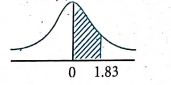
(a) lies between 0 and 1.83
(b) is greater than 1.54
(c) is greater than -0.86
(d) lies between 0.43 and 1.12
(e) is less than 0.77
4.
Let X denote the number of hours you study during a randomly selected school day. The probability that X can take the value X has the following form, where k is some unknown constant \(p(X=x)= \begin{cases}0.1 & \text { if } x=0 \\ k x & \text { if } x=1 \text { or } 2 \\ k(5-x) & \text { if } x=3 \text { or } 4 \\ 0 & \text { otherwise }\end{cases}\)
(i) Find the value of k
(ii) What is the probability that you study atleast 2 hours?
(iii) Exactly 2 hours
(iv) At most 2 hours
5.
From the data find the number of students whose height is between 80 cm and 90 cm.
| Height in cm's | 40-60 | 60-80 | 80-100 | 100-120 | 120-140 |
| No. of students y | 240 | 120 | 100 | 70 | 50 |
6.
Integrate \(\int{\sqrt{1-sin2x}dx }\)
7.
The net profit p and quantity x satisfy the differential equation \(\frac{d p}{d x}=\frac{2 p^{3}-x^{3}}{3 x p^{2}}\). Find the relationship between net profit and demand given that p = 20, when x = 10.
8.
Find the area of the region \(\left\{(x, y) ; x^{2} \leq y \leq|x|\right\} .\)
9.
Evaluate \(\int\left[\frac{2+x+x^{2}}{x^{2}(2+x)}+\frac{2 x-1}{(x+1)^{2}}\right] d x\)
10.
Find k if the equation x + 2y 3 = -2, 3x - y - 2z = 1 and 2x + 3y 5z = k are consistent
11.
Calculate Fisher's ideal index from the following data and verify that it satisfies both time reversal and factor reversal test
| Commodity | Price | Quantity | ||
| 1985 | 1986 | 1985 | 1986 | |
| A | 8 | 20 | 50 | 60 |
| B | 2 | 6 | 15 | 10 |
| C | 1 | 2 | 20 | 25 |
| D | 2 | 5 | 10 | 8 |
| E | 1 | 5 | 40 | 30 |
12.
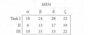
Solve the following assignment problem.
13.
The area A of circle of diameter ‘d’ is given for the following values
| D | 80 | 85 | 90 | 95 | 100 |
| A | 5026 | 5674 | 6362 | 7088 | 7854 |
Find the approximate values for the areas of circles of diameter 82 and 91 respectively
14.
The following data are taken from the steam table
| Temperature C0 | 140 | 150 | 160 | 170 | 180 |
| Pressure kg f / cm2 | 3.685 | 4.854 | 6.302 | 8.076 | 10.225 |
Find the pressure at temperature t = 1750
15.
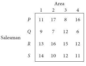
Find the optimal solution for the assignment problem with the following cost matrix.
16.
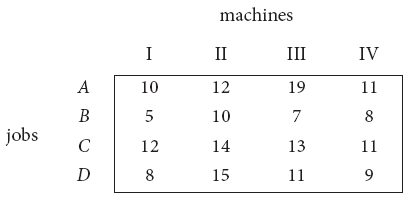
Solve the following assignment problem. Cell values represent cost of assigning job A, B, C and D to the machines I, II, III and IV.
17.
(D2 − 3D + 2)y = e3x which shall vanish for x = 0 and for x = log 2
18.
A machine is set to deliver packets of a given weight. Ten samples of size five each were recorded. Below are given relevant data:
| Sample number | 1 | 2 | 3 | 4 | 5 | 6 | 7 | 8 | 9 | 10 |
| \(\overset {-}{X}\) | 15 | 17 | 15 | 18 | 17 | 14 | 18 | 15 | 17 | 16 |
| R | 7 | 7 | 4 | 9 | 8 | 7 | 12 | 4 | 11 | 5 |
Calculate the control limits for mean chart and the range chart and then comment on the state of control. (conversion factors for n = 5, A2 = 0.58, D3 = 0 and D4 = 2.115
19.
The following table shows the number of salesmen working for a certain concern:
| Year | 1992 | 1993 | 1994 | 1995 | 1996 |
| No. of salesmen | 46 | 48 | 42 | 56 | 52 |
Use the method of least squares to fit a straight line and estimate the number of salesmen in 1997.
20.
The marginal revenue ‘y’ of output ‘q’ is given by the equation \(\frac { dy }{ dq } =\frac { { q }^{ 2 }+{ 3 }y^{ 2 } }{ 2qy } \). Find the total Revenue function when output is 1 unit and Revenue is Rs. 5.
21.
The average score on a nationally administered aptitude test was 76 and the corresponding standard deviation was 8. In order to evaluate a state’s education system, the scores of 100 of the state’s students were randomly selected. These students had an average score of 72. Test at a significance level of 0.05 if there is a significant difference between the state scores and the national scores.
22.
Using the following random number table,
| Tippet’s random number table | |||||||
| 2952 | 6641 | 3992 | 9792 | 7969 | 5911 | 3170 | 5624 |
| 4167 | 9524 | 1545 | 1396 | 7203 | 5356 | 1300 | 2693 |
| 2670 | 7483 | 3408 | 2762 | 3563 | 1089 | 6913 | 7991 |
| 0560 | 5246 | 1112 | 6107 | 6008 | 8125 | 4233 | 8776 |
| 2754 | 9143 | 1405 | 9025 | 7002 | 6111 | 8816 | 6446 |
Draw a sample of 10 children with their height from the population of 8,585 children as classified here under.
| Height (cm) | 105 | 107 | 109 | 111 | 113 | 115 | 117 | 119 | 121 | 123 | 125 |
| Number of children | 2 | 4 | 14 | 41 | 83 | 169 | 394 | 669 | 990 | 1223 | 1329 |
| Height(cm) | 127 | 129 | 131 | 133 | 135 | 137 | 139 | 141 | 143 | 145 | |
| No. of children | 1230 | 1063 | 646 | 392 | 202 | 79 | 32 | 16 | 5 | 2 |
23.
The annual salaries of employees in a large company are approximately normally distributed with a mean of Dallor. 50,000 and a standard deviation of Dallor.20,000.
(a) What percent of people earn less than Dallor.40,000?
(b) What percent of people earn between Dallor.45,000 and Dallor.65,000?
(c) What percent of people earn more than Dallor.70,00
24.
The marks obtained in a certain exam follow normal distribution with mean 45 and SD 10. If 1,300 students appeared at the examination, calculate the number of students scoring
(i) less than 35 marks and
(ii) more than 65 marks.
25.
Evaluate \(\int\left[\frac{1}{\log x}-\frac{1}{(\log x)^{2}}\right] d x\)
26.
Suppose that the time in minutes that a person has to wait at a certain station for a train is found to be a random phenomenon with a probability function specified by the distribution function\(F(x)\begin{cases} 0,\quad \text{for}\quad x<0 \\ \frac { 1 }{ 2 } ,\quad \text{for}\quad 0\le x<1 \\ 0,\quad \text{for}\quad 1\le x<2\quad \\ \frac { 1 }{ 4 } ,\quad \text{for}\quad 2\le x<4 \\ 0,\quad \text{for}\quad x\ge 4 \end{cases}\)
(a) Is the distribution function continuous? If so, give its probability density function?
(b) What is the probability that a person will have to wait
(i) more than 3 minutes,
(ii) less than 3 minutes and
(iii) between 1 and 3 minutes?
27.
A firm’s marginal revenue function is MR = 20e-x/10 \(\left( 1-\frac { x }{ 10 } \right) \). Find the corresponding demand function.
28.
The amount of bread (in hundreds of pounds) x that a certain bakery is able to sell in a day is found to be a numerical valued random phenomenon, with a probability function specified by the probability density function f(x) is given by
\(f(x)=\left\{\begin{array}{l} Ax,for \ 0≤x10 \\ A(20−x),for \ 10 ≤x< 20 \\ 0,\quad \quad \quad otherwise \end{array}\right.\)
(a) Find the value of A.
(b) What is the probability that the number of pounds of bread that will be sold tomorrow is
(i) More than 10 pounds,
(ii) Less than 10 pounds, and
(iii) Between 5 and 15 pounds?
29.
In a market survey three commodities A, B and C were considered. In finding out the index number some fixed weights were assigned to the three varieties in each of the commodities. The table below provides the information regarding the consumption of three commodities according to the three varieties and also the total weight received by the commodity
| Commodity Variety | Variety | Total weight | ||
| I | II | III | ||
| A | 1 | 2 | 3 | 11 |
| B | 2 | 4 | 5 | 21 |
| C | 3 | 5 | 6 | 27 |
Find the weights assigned to the three varieties by using Cramer’s Rule.
30.
Find k, if the equations x + y + z = 7, x + 2y + 3z = 18, y + kz = 6 are inconsistent
1.
I(x) = 200 –0.2x C1 = ₹ 3.5 T = 30 Total inventory carrying cost = 20,685
2.
\(\mathrm{n}=400,\ \bar{x}=171.38, \ \sigma=3.3\)
Null Hypothesis :
\(\mathrm{H}_{0}: \mu=171.17\)
Alternative Hypothesis :
\(\mathrm{H}_{1}: \mu \neq 171.17\)
Test statistic :
\( \mathrm{Z} =\frac{\bar{x}-\mu}{\frac{\sigma}{\sqrt{n}}} \sim N(0,1) \)
\(=\frac{171.38-171.17}{\frac{3.3}{\sqrt{400}}}=1.273 \)
Since |z| = 1.273 < 1.96 we accept null hypothesis at 5% level of significance. Thus the sample of 400 has come from the population with height of 171.17 cms
3.
\(\text {(a) } \mathrm{P}(0 \leq Z \leq 1.83)=0.4664\)
\(\text {(b) } \mathrm{P}(Z \geq 1.154)\)
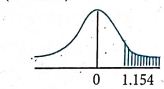
\( =0.5-p(0 \leq Z \leq 1.154) \)
\(=0.5-0.4382=0.0618\)
\(\text {(c) } \mathrm{P}(Z \geq-0.86)\)
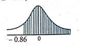
\( =0.5+\mathrm{P}(-0.86 \leq \mathrm{Z} \leq 0) \)
\(=0.5+0.3051=0.8051\)
\(\text {(d) } \mathrm{P}^{\prime}(0.43 \leq Z \leq 1.12)\)
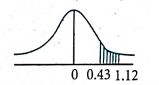
\( =\mathrm{P}(0 \leq Z \leq 1.12)-\mathrm{P}(0 \leq Z \leq 0.43) \)
= 0.3686-0.1664
= 0.2022
\(\text {(e) } \mathrm{P}(\mathrm{Z} \leq 0.77)=0.5+\mathrm{P}(0 \leq Z \leq 0.77)\)
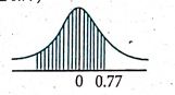
= 0.5 + 0.2794
= 0.7794
4.
(i) The Probability distribution of X
| x | 0 | 1 | 2 | 3 | 4 |
| p(x) | 0.1 | k | 2k | 2k | k |
\(
\sum P_{i} =1
\)
\(0.1+\mathrm{k}+2 \mathrm{k}+2 \mathrm{k}+\mathrm{k} =1
\)
\(6 \mathrm{k} =1-0.1
\)
\(6 \mathrm{k} =0.9 \Rightarrow \mathrm{k}=0.15
\)
(ii) \(\mathrm{P}(x \geq 2)=\mathrm{P}(\mathrm{X}=2)+\mathrm{P}(\mathrm{X}=3)+\mathrm{P}(\mathrm{X}=4)\)
2k + 2k +k = 5k
= 5(0.15) = 0.75
(iii) P(X = 2) = 2k = 2(0.15) = 0.3
(iv) \(\mathrm{P}(x \leq 2)=\mathrm{P}(\mathrm{X}=0)+\mathrm{P}(\mathrm{X}=1)+\mathrm{P}(\mathrm{X}=2)\)
0.1 + k + 2k = 0.1 + 3k
= 0.1 + 3(0.15) = 0.55
5.
\( x_{0} =60, \mathrm{~h}=20, x_{0}+\mathrm{nh}=90 \\ 20 \mathrm{n} =30 \Rightarrow \mathrm{n}=1.5 \)
| x | y | \(\nabla y\) | \(\Delta^{2} y\) | \(\Delta^{3} y\) | \(\Delta^{4} y\) |
| Below 60 | 250 | ||||
| 120 | |||||
| Below 80 | 370 | -20 | |||
| 100 | -10 | ||||
| Below 100 | 470 | -30 | 20 | ||
| 70 | 10 | ||||
| Below 120 | 540 | -20 | |||
| 50 | |||||
| Below 140 | 590 |
\( y=y_{0}+\frac{n}{1 !} \Delta y_{6}+\frac{n(n-1)}{2 !} \Delta^{2} y_{0}+\frac{n(n-1)(n-2)}{3 !} \Delta^{3} y_{0}
\) \(+\frac{n(n-1)(n-2)(n-3)}{4 !} \Delta^{4} y_{0} \)
\( y(90)= 250+\frac{(1.5)}{1 !}(250)+\frac{(1.5)(1.5-1)}{2 !}(-20) +\frac{(1.5)(1.5-1)(1.5-2)}{3 !}(-10)+\frac{(1.5)(1.5-1)(1.5-2)(1.5-3)}{4 !}(20)\)
= 250+180.7 .5+0.625+0.46875
\(
=423.59 \sim 424
\)
6.
-cosx-sinx+c
7.
\(\frac{d p}{d x}=\frac{2 p^{3}-x^{3}}{3 x p^{2}}\)
It is a differential equation in x and p of homogeneous type.
\(
\therefore \mathrm{p} =\mathrm{v} x \\
\frac{d p}{d x} =v+x \frac{d v}{d x}
\)
\(v+x \frac{d v}{d x} =\frac{2 v^{3} x^{3}-x^{3}}{3 x\left(v^{2} x^{2}\right)}=\frac{2 v^{3}-1}{3 v^{2}}
\)
\(x \frac{d v}{d x} =\frac{2 v^{3}-1}{3 v^{2}}-v
\)
\( =\frac{2 v^{3}-1-3 v^{3}}{3 v^{2}}=-\left(\frac{1+v^{3}}{3 v^{2}}\right)
\)
\(\int \frac{3 v^{2}}{1+v^{3}} d v =-\int \frac{d x}{x}
\)
\(\log \left(1+v^{3}\right) =-\log x+\log \mathrm{c}
\)
\(\log \left(1+\frac{p^{3}}{x^{3}}\right)+\log x =\log \mathrm{c} \)
\(\log \left(\frac{x^{3}+p^{3}}{x^{3}}\right) x =\log \mathrm{c}
\)
\(x^{3}+\mathrm{p}^{3} =c^{2} \)
\(\text {If } \mathrm{p} =20, x=10
\)
\(
1000+8000 =c(100)
\)
\(\Rightarrow =\frac{9000}{100}=90
\)
Required equation is \(x^{3}+\mathrm{p}^{3}=90 x^{2}\)
8.
y = x2 is a parabola open upwards
\(
\mathrm{y} =|x| \Rightarrow \mathrm{y}=x \text { if } x \geq 0
\)
\(=-x \text { if } x<0
\)
Since the curve is symmetrical about y-axis
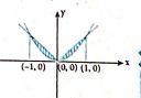
\(
\text {Area } =\int_{a}^{b} y d x \\
=2 \int_{0}^{1}\left(x-x^{2}\right) d x
\)
\( =2\left[\frac{x^{2}}{2}-\frac{x^{3}}{3}\right]_{0}^{1}=2\left[\frac{1}{2}-\frac{1}{3}\right]
\)
\( =2\left(\frac{3-2}{6}\right)=\frac{1}{3} \text { sq. units }
\)
9.
\( \int\left[\frac{2+x+x^{2}}{x^{2}(2+\mathrm{x})}+\frac{2 x-1}{(\mathrm{x}+1)^{2}}\right] d x \)
\( =\int\left[\frac{2+x}{x^{2}(2+\mathrm{x})}+\frac{x^{2}}{\mathrm{x}^{2}(2+x)}+\frac{2(\mathrm{x}+1)-3}{(\mathrm{x}+1)^{2}}\right] d x \)
\( =\int\left[\frac{1}{x^{2}}+\frac{1}{2+x}+\frac{2}{\mathrm{x}+1}-\frac{3}{(\mathrm{x}+1)^{2}}\right] d x \)
\(=\int\left[x^{-2}+\frac{1}{2+x}+\frac{2}{x+1}-3(\mathrm{x}+1)^{-2}\right] d x \)
\(=\frac{x^{-1}}{-1}+\log |2+x|+2 \log |x+1|-\frac{3(x+1)^{-1}}{-1}+c \)
\(=\frac{-1}{x}+\log |2+x|+2 \log |\mathrm{x}+1|+\frac{3}{(\mathrm{x}+1)}+c\)
10.
In matrix form
\(\left(\begin{array}{ccc}
1 & 2 & -3 \\
3 & -1 & -2 \\
2 & 3 & -5
\end{array}\right)\left(\begin{array}{l}
x \\
y \\
z
\end{array}\right)=\left(\begin{array}{c}
-2 \\
1 \\
k
\end{array}\right)\)
AX = B
Augmented matrix
\((A, B)=\left(\begin{array}{cccc}
1 & 2 & -3 & -2 \\
3 & -1 & -2 & 1 \\
2 & 3 & -5 & k
\end{array}\right)\)
\(\sim\left(\begin{array}{cccc}
1 & 2 & -3 & -2 \\
0 & -7 & 7 & 7 \\
0 & -1 & 1 & K+4
\end{array}\right) \begin{aligned}
&R_{2} \rightarrow R_{2}-3 R_{1} \\
&R_{3} \rightarrow R_{3}-2 R_{1}
\end{aligned}\)
\(\sim\left(\begin{array}{cccc}
1 & 2 & -3 & -2 \\
0 & -1 & 1 & 1 \\
0 & -1 & 1 & k+4
\end{array}\right) \quad R_{2} \rightarrow R_{2} / 7\)
\(\sim\left(\begin{array}{cccc}
1 & 2 & -3 & -2 \\
0 & -1 & 1 & 1 \\
0 & 0 & 0 & k+3
\end{array}\right) \quad R_{3} \rightarrow R_{3}-R_{2}\)
Since the system is consistent
\(\rho(A, B)=\rho(A)=2\)
k + 3 = 0
k = -3
11.
| Commodity | 1985 | 1986 | ||
| p0 | q0 | p1 | q1 | |
| A | 8 | 50 | 20 | 60 |
| B | 2 | 15 | 6 | 10 |
| C | 1 | 20 | 2 | 25 |
| D | 2 | 10 | 5 | 8 |
| E | 1 | 40 | 5 | 30 |
| p1q0 | p0q0 | p1q1 | p0q1 |
| 1000 | 410 | 1200 | 480 |
| 90 | 30 | 60 | 20 |
| 40 | 20 | 50 | 25 |
| 50 | 20 | 40 | 16 |
| 200 | 40 | 150 | 30 |
| 1380 | 510 | 1500 | 571 |
Fisher's Ideal Index = \(\sqrt\frac{{\Sigma p_1q_0}\times{\Sigma p_1q_1}}{{\Sigma p_0q_0}\times{\Sigma p_0q_1}}\times100\)
\(= \sqrt\frac{1380\times1500}{510\times571}\times100\)
= 266.61
Time reversaltest:
\(P_{01}\times P_{10}=\sqrt\frac{{\Sigma p_1q_0}\times{\Sigma p_1q_1}\times{\Sigma p_0q_1}\times{\Sigma p_0q_0}}{{\Sigma p_0q_0}\times{\Sigma p_0q_1}\times{\Sigma p_1q_1}\times{\Sigma p_1q_0}}\)
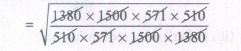
= \(\sqrt{1}=1\)
Hence, time reversal test is satisfied.
Factor reversaltest:
\(P_{01}\times Q_{01}=\sqrt\frac{{\Sigma p_1q_0}\times{\Sigma p_1q_1}\times{\Sigma q_1p_0}\times{\Sigma q_1p_1}}{{\Sigma p_0q_0}\times{\Sigma p_0q_1}\times{\Sigma q_0p_0}\times{\Sigma q_0p_1}}\)

\(P_{01}\times Q_{01}=\frac{{\Sigma p_1q_1}}{{\Sigma p_0q_0}}\)
Hence, Fisher's ideal index satisfies factor reversal test also.
12.
Since the number of rows is less then the number of columns, given assignment problem is unbalanced one.
To balance it, introduce a dummy row with all the entries zero.
The revised assignment problem is
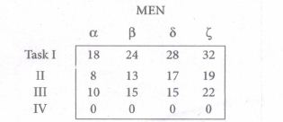
Here only 3 tasks can be assigned to 3 men.
Step 1 :
Select the smallest element in each row and subtract it will all the elements in its row.
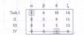
Here each row and column has atleast one zero.
Step 2:
Examine the row with only one zero, mark that zero by \(\Box\) and draw a vertical line.
After examining all the rows, examine the column with single zero, mark that zero by \(\Box\) and draw a horizontal line.
Step 3:
Only two assignment have been made.
The elements not lying on the line are
\(\begin{matrix} 6 & 10 & 14 \\ 5 & 9 & 11 \\ 5 & 5 & 12 \end{matrix}\)
and minimum is 5.
Subtract 5 from all these numbers. Other numbers remains the same.
A new cost matrix will be found .and repeat step 2.
∴ The new cost matrix is
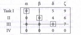
Thus, 3 assignments have been made.
The optical assignment schedule and total cost is
| Task | MEN | Cost |
| I | α | 18 |
| II | β | 13 |
| III | δ | 15 |
| Total Cost | Rs. 46 | |
13.
Let the diameter be x and area be y.
To find y when x = 82, use Newton's forward interpolation form
∴ x0 + nh = 82 ⇒ 80 + n(5) ⇒ 82 - 80 = 2
⇒ n = \(\frac{2}{5}\) = 0.4
The difference table is
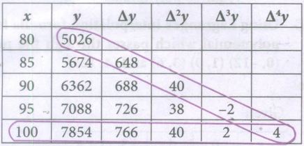
∴ y(82) = y0 + \(\frac { n }{ 1! } { \triangle y }_{ 0 }+\frac { n(n+1) }{ 2! } { \triangle }^{ 2 }{ y }_{ 0 }+\frac { n(n+1)(n+2) }{ 3! } { \triangle }^{ 3 }{ y }_{ 0 }\)+ \(\frac { n(n+1)(n+2)(n-3) }{ 4! } { \triangle }^{ 4 }{ y }_{ 0 }\)
.JPG)
+ \(\frac{(0.4)(0.4-1)(0.4-2)}{6}\)(-2)
.JPG)
= 5026 + 259.2 + (0.4) (-0.6) (20) + \(\frac{(0.4)(-0.6)(-1.6)(-1)}{3}\) + \(\frac{(0.4)(-0.6)(-1.6)(-2.6)}{3}\)
= 5026 + 259.2 - 4.8 - 0.128 - 0.1664
= 5280.10
∴ When the diameter is 82, area of circle is 5280.1 (≅ 5281)
To find y when x = 91, use Newton's backward interpolation formula.
∴ xn + nh = 91 ⇒ 100 + n(5) = 91
⇒ 5n = 91 - 100
⇒ 5n = -9 ⇒ n = \(\frac{-9}{5}\) = 1.8
Newton's backward interpolation formula is
y(x=xn+nh) = yn + \(\frac { n }{ 1! } \triangledown { y }_{ n }+\frac { n(n+1) }{ 2! } { \triangledown }^{ 2 }{ y }_{ n }+\frac { n(n+1)(n+2) }{ 3! } { \triangledown }^{ 3 }{ y }_{ n }\)
y(x = 91) = 7854 - 1.8 (766) +
.JPG)
\(+\frac{(-1.8)(-1.8+1)(-1.8+2)(-1.8+3)}{3!}\)(4)
⇒ y(x = 91) = 7854 - 1378.8 + (-1.8) (-0.8) (20) + (-1.8) (-0.8) (0.2) + \(\frac{(-1.8)(-0.8)(0.2)(1.2)}{6}\) (4)
⇒ y(x = 91) = 7854 - 1378.8 + 28.8 + 0.288 + 0.2304
⇒ y(x = 91) = 6504.5
Hence when the diameter is 91, area is 6504.5 ≅ 6504
14.
Since the pressure required is at the end of the table, we apply Backward interpolation formula. Let temperature be x and the pressure be y.
\({ y }_{ \left( x={ x }_{ 0 }+nh \right) }={ y }_{ 0 }+\frac { n }{ n! } \Delta { y }_{ 0 }+\frac { n(n-1) }{ 2! } { \Delta }^{ 2 }{ y }_{ 0 }+\frac { n(n-)(n-2) }{ 3! } { \Delta }^{ 3 }{ y }_{ 0 }+...\)
To find y at x = 175
\(\therefore\) xn + nh = 175 , xn = 180, h = 10 \(\Rightarrow\) n = −0.5
| x | y | \(\Delta y\) | \(\Delta ^{ 2 }y\) | \(\Delta ^{ 2 }y\) | \(\Delta ^{ 4 }y\) |
| 140 | 3.685 | ||||
| 1.169 | |||||
| 150 | 4.854 | 0.279 | |||
| 1.448 | 02.047 | ||||
| 160 | 6.032 | 0.326 | 0.002 | ||
| 1.774 | 0.049 | ||||
| 170 | 8.076 | 0.375 | |||
| 2.149 | |||||
| 180 | 10.225 |
\({ y }_{ (x=1750 }=10.225+\left( -0.5 \right) (2.149)+\frac { (-0.5)(0-5) }{ 2! } (0.375)+\frac { (-0.5)(0-5)(1.5) }{ 3! } (0.049)+\frac { (-0-5)(0.5)(1.5)(2.5) }{ 4! } (0.002)\)
= 10.225−1.0745−0.046875−0.0030625 − 0.000078125
= 9.10048438
= 9.1
15.
Here, the number of rows and columns are equal.
∴ The given assignment problem is balanced.
Step 1 : Select a smallest element in each row and subtract this from all the elements in its row.
∴ The cost matrix: of the given assignment problem is
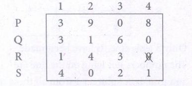
Column 1 contains no zero. Go to step 2.
Step 2 : Select the smallest element (1) in column 1 and subtract this from all the elements in its column.
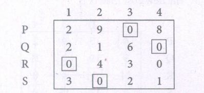
Since each row and column contains atleast one zero, assignments can be made.
Step 3 : Examine the rows with only one zero.
Row P, Q and S contains exactly one zero, mark them by 0 and mark the other zeros in the column byX.
Thus, all the four assignments have been made.
∴ The optimal assignment schedule and total cost is
| Salesman | Area | Cost |
|---|---|---|
| P | 3 | 8 |
| Q | 4 | 6 |
| R | 1 | 13 |
| S | 2 | 10 |
| Total Cost | Rs. 37 | |
16.
Here the number of rows and columns are equal.
\(\therefore\)The given assignment problem is balanced.
Now let us find the solution.
Step 1: Select a smallest element in each row and subtract this from all the elements in its row.
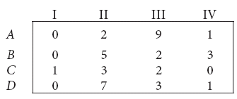
Look for atleast one zero in each row and each column.Otherwise go to step 2.
Step 2 : Select the smallest element in each column and subtract this from all the elements in its column.
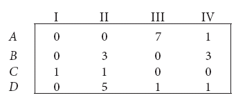
Since each row and column contains atleast one zero, assignments can be made.
Step 3 (Assignment):
Examine the rows with exactly one zero. First three rows contain more than one zero. Go to row D.
There is exactly one zero. Mark that zero by \(\square\) (i.e) job D is assigned to machine
I . Mark other zeros in its column by\(\text { X }\).
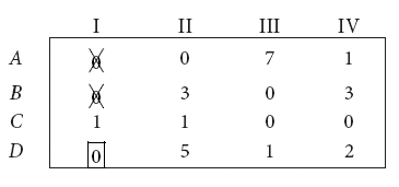
Step 4: Now examine the columns with exactly one zero. Already there is an assignment in column I. Go to the column II. There is exactly one zero. Mark that zero by \(\square\) . Mark other zeros in its row by\(\text { X }\).
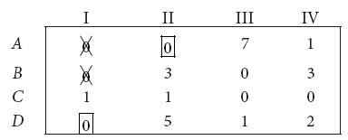
Column III contains more than one zero. Therefore proceed to Column IV, there is exactly one zero. Mark that zero by \(\square\) . Mark other zeros in its row by \(\text { X }\).
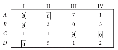
Step 5: Again examine the rows. Row B contains exactly one zero. Mark that zero by \(\square\).
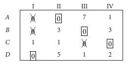
Thus all the four assignments have been made. The optimal assignment schedule and total cost is
\(\begin{array}{|c|c|c|} \hline \text { Job } & \text { Machine } & \text { cost } \\ \hline \text { A } & \text { II } & 12 \\ \hline \text { B } & \text { III } & 7 \\ \hline \text { C } & \text { IV } & 11 \\ \hline \text { D } & \text { I } & 8 \\ \hline {\text { Total cost }} \ && 38 \\ \hline \end{array}\)
The optimal assignment (minimum) cost
= Rs. 38
17.
Auxiliary equation is m2 - 3m + 2 = 0
∴ (m - 1)(m - 2) = 0
⇒ m = 1,2
∴ Complementary function CF is Aex + Be2x
PI = \(\frac { 1 }{ \phi (D) } \)(x)
= \(\frac { 1 }{ { D }^{ 2 }-3D+2 } \).e3x
= \(\frac { 1 }{ (D-1)(D-2) } \).e3x
= \(\frac { e^{ 3x } }{ (3-1)(3-2) } \).e3x
= \(\frac { { e }^{ 3x } }{ 2 } \)
General solution is y = CF + PI
y = Aex+Be2x+\(\frac { 1 }{ 2 } \)e3x ...(1)
Given when x = 0, y = 0
∴ 0 = Ae0+Be0+\(\frac { 1 }{ 2 } \)e0 ⇒ 0 = A+B-\(\frac { 1 }{ 2 } \) ..(2)
Also, when x = log2, y = 0
⇒ 0 = Aelog2+Be2log2+e3log3
⇒ 0 = A(2)+\(Be^{ log2^{ 2 }+ }+\frac { 1 }{ 2 } elog2^{ 3 }\)
⇒ 0 = 2A+4B+\(\frac{8}{2}\) ⇒ 2A+4B=-4
⇒ A+2B = -2
(2)-(3) ⇒ A+B = -\(\frac { 1 }{ 2 } \)
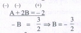
Substituting B = -\(\frac { 3 }{ 2 } \) in (2) we get
\(A-\frac { 3 }{ 2 } =-\frac { 1 }{ 2 } \Rightarrow A=-\frac { 1 }{ 2 } +\frac { 3 }{ 2 } \Rightarrow \frac { 2 }{ 2 } \)=1
∴ y = \(1.e^{ x }-\frac { 3 }{ 2 } e^{ 2x }+\frac { e^{ 3x } }{ 2 } \).
18.
| Sample No | \(\overline {X}\) | R |
| 1 | 15 | 7 |
| 2 | 17 | 7 |
| 3 | 15 | 4 |
| 4 | 18 | 9 |
| 5 | 17 | 8 |
| 6 | 14 | 7 |
| 7 | 18 | 12 |
| 8 | 15 | 4 |
| 9 | 17 | 11 |
| 10 | 16 | 5 |
\(\overline {\overline {X}} = \frac{15+17+15+18+17+14+18+15+17+15+17+16}{10}\) = \(\frac {162}{10}\) = 16.2
\(\overline {R}\) = \(\frac{7 + 7 + 4+ 9+ 8+ 12 + 7 + 4+ 11+ 15}{10}\) = \(\frac {74}{10}\) = 7.4
Control limits for mean chart
UCL = \(\overline {\overline{X}} + A_{2} \overline {R}\)
= 16.2 + 0.58(7.4)
= 16.2 + 4.292 = 20.492
[∴ A2 = 0.58]
CL = \(\overline {\overline{X}}\) = 16.2
LCL = \(\overline {\overline{X}} - A_{2} \overline {R}\)
= 16.2 - 0.58(7.4)
= 16.2 - 4.292 = 11.91
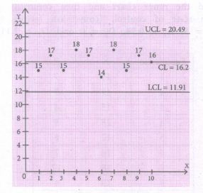
Control limits for R-chart
UCL = D4 \(\overline{R}\)
= 2.115 (7.4) = 15.65
[∴ D4 = 2.115]
CL = \(\overline{R}\) = 7.4
LCL = D3 \(\overline{R}\)
= 0(\(\overline{R}\)) = 0
[∴ D3 = 0]
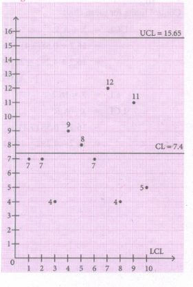
Conclusion : The above diagram shows all the control lines with the data points plotted. Since all the points lie within the control limits, we can say that the process is in control.
19.
| Year (X) | No. of Salesmen Y | X = x -1994 | X2 | XY |
| 1992 | 46 | -2 | 4 | -92 |
| 1993 | 48 | -1 | 1 | -48 |
| 1994 | 42 | 0 | 0 | 0 |
| 1995 | 56 | 1 | 1 | 56 |
| 1996 | 52 | 2 | 4 | 104 |
| 244 | 0 | 10 | 20 |
Smce \(\sum\)X = 0, a =\(\frac {\sum Y}{n}\) = \(\frac {244}{5}\) = 48.8
b = \(\frac {\sum XY}{\sum X^2}\) = \(\frac {20}{10}\) = 2
∴ The required equation of the straight line trend is given by
Y = a + bX \(\Rightarrow \) Y = 48.8 + 2X
\(\Rightarrow \) Y = 48.8 +2 (X - 1994) .... (1)
∴ Number of salesmen in 1997 is put X = 1997 in (1)
∴ Y = 48.8 + 2 (1997 - 1994)
= 48.8 + 2 (3)
= 48.8 + 6 = 54.8
∴ Number of salesmen in 1997 is 54.8
20.
Given that \(MR=\frac { dy }{ dq } =\frac { { q }^{ 2 }+{ 3 }y^{ 2 } }{ 2qy } \) (1)
Put y = vq and \(\frac { dy }{ dq } =v+q\frac { dv }{ dq } \) in (1)
Now (1) becomes
\(v+q\frac { dy }{ dq } =\frac { { q }^{ 2 }+{ 3 }v^{ 2 }{ q }^{ 2 } }{ 2yvq } \)
\(=\frac { 1+3{ v }^{ 2 } }{ 2v } \)
\(q\frac { dv }{ dq } =\frac { 1+3{ v }^{ 2 } }{ 2v } -v\)
\(=\frac { 1+3{ v }^{ 2 }-2{ v }^{ 2 } }{ 2v } \)
\(=\frac { { 1+v }^{ 2 } }{ 2v } \)
\(\frac { 2v }{ { 1+v }^{ 2 } } dv=\frac { dq }{ q } \)
On Integration
\(ഽ\frac { 2v }{ { 1+v }^{ 2 } } dv=ഽ\frac { dq }{ q } \)
log (1+ v2) = log q + log c
1+ v2 = cq
Replace \(v=\frac { y }{ q } \)
\(1+\frac { { y }^{ 2 } }{ { q }^{ 2 } } \) = cq
q2 + y2 = c q3 (2)
Given output is 1 unit and revenue is Rs. 5
∴ (2) ⇒ 1 + 25 = c ⇒ c = 26
∴ The total revenue function is q2 + y2 = 26q3
21.
Sample size n = 100
Sample mean \(\bar { X } \)= 72
Population mean μ = 76
Population standard deviation σ = 8
Null Hypotheses H0:
μ = 76(i.e., There is no Significant difference between the state scores and the national scores)
\(Z=\frac { \bar { X } -\mu }{ \frac { \sigma }{ \sqrt { n } } } \)
\(\Rightarrow Z=\frac { 72-76 }{ \frac { 8 }{ \sqrt { 100 } } } =\frac { -4 }{ \frac { 8 }{ 10 } } =\frac { -4 }{ 8 } =-5\)
\(\Rightarrow |Z|=5\)
\({ Z }_{ \frac { \alpha }{ 2 } }=1.96\)
\(Z>{ Z }_{ \frac { \alpha }{ 2 } }i.e.,\ 5>1.96\)
Inference : Since \(Z>{ Z }_{ \frac { \alpha }{ 2 } }\) at 5% level of significance, the null hypothesis H0 is rejected.
Hence, we conclude that there is significant difference between the state scores and the national scores.
22.
The first thing is to number the population (8585 children). The numbering has already been provided by the frequency table. There are 2 children with height of 105 cm, therefore we assign number 1 and 2 to the children those in the group 105 cm, number 3 to 6 is assigned to those in the group 107 cm and similarly all other children are assigned the numbers. In the last group 145 cms there are two children with assigned number 8584 and 8585.
| Height (cm) | Number of children | Cumulative Frequency |
| 105 | 2 | 2 |
| 107 | 4 | 6 |
| 109 | 14 | 20 |
| 111 | 41 | 61 |
| 113 | 83 | 144 |
| 115 | 169 | 313 |
| 117 | 394 | 707 |
| 119 | 669 | 1376 |
| 121 | 990 | 2366 |
| 123 | 1223 | 3589 |
| 125 | 1329 | 4918 |
| 127 | 1230 | 6148 |
| 129 | 1063 | 7211 |
| 131 | 646 | 7857 |
| 133 | 392 | 8249 |
| 135 | 202 | 8451 |
| 137 | 79 | 8530 |
| 139 | 32 | 8562 |
| 141 | 16 | 8578 |
| 143 | 5 | 8583 |
| 145 | 2 | 8585 |
| Total | 8585 |
Now we take 10 samples from the tables, since the population size is in 4 digits we can use the given random number table. Select the10 random numbers from 1 to 8585 in the table, Here, we consider column wise selection of random numbers, starting from first column.
| Tippet’s random number table | |||||||
| 2952 | 6641 | 3992 | 9792 | 7969 | 5911 | 3170 | 5624 |
| 4167 | 9524 | 1545 | 1396 | 7203 | 5356 | 1300 | 2693 |
| 2670 | 7483 | 3408 | 2762 | 3563 | 1089 | 6913 | 7991 |
| 0560 | 5246 | 1112 | 6107 | 6008 | 8125 | 4233 | 8776 |
| 2754 | 9143 | 1405 | 9025 | 7002 | 6111 | 8816 | 6446 |
The children with assigned number 2952 is selected and then see the cumulative frequency table where 2952 is present, now select the corresponding row height which is 123 cm, similarly all the selected random numbers are considered for the selection of the child with their corresponding height. The following table shows all the selected 10 children with their heights.
| Child with assigned Number | 2952 | 4167 | 2670 | 0560 | 2754 |
| Corresponding Height (cms) | 123 | 125 | 123 | 117 | 123 |
| Child with assigned Number | 6641 | 7483 | 5246 | 3996 | 1545 |
| Corresponding Height (cms) | 129 | 131 | 127 | 125 | 121 |
23.
(a) P(X<40,000)
When X = 40,000.
Z = \(\frac { X-\mu }{ \sigma } \)
= \(\frac { 40,000-50,000 }{ 20,000 } \) = -0.5
∴ P(X<40,000) = P(Z<-0.5)
= P(-∞
= 0.5-0.1915 = 0.3085
∴ 30.85 % pf people earn less than $40,000
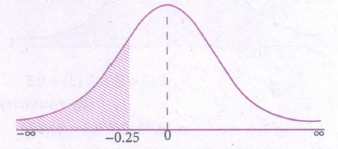
(b) P(45,000 < X < 65,000)
When X = 45,000
Z1 = \(\frac { 45,000-50,000 }{ 20,000 } \) = -0.25
When X=65,000
Z=\(\frac { 65,000-50,000 }{ 20,000 } \)=0.75
∴ P(45000 < X < 65,000) = P(-0.25 < Z < 0.75)
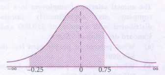
= P (-0.25 < Z < 0) + P(0 < Z < 0.75)
= P(0 < Z < 0.25) + P (0 < Z < 0.75)
= 0.0987 + 0.2734 = 0.3721
Hence, 37.21% of people earn between Dallor 45,000 and Dallor 65,000.
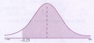
(c) P(X>7000)
When X = 7000
Z = \(\frac { 75000-50,000 }{ 20,000 } \) = 1.25
∴ P(X > 7000) = P(Z > 1.25)
= 0.5 - 0.3944
= 0.1056
24.
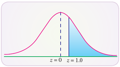
Let X be the normal variate showing the score of the candidate with mean 45 and standard deviation 10.
(i) less than 35 marks
When X = 35
\(Z=\frac { X-\mu }{ \sigma } =\frac { 35-45 }{ 10 } =-1\)
P(X < 35) = P(Z < –1)
P(Z > 1) = 0.5 – P(0 < Z < 1)
= 0.5 – 0.3413
= 0.1587
Expected number of students scoring less than 35 marks are 0.1587 × 1300
= 206
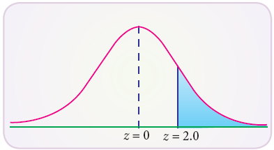
(ii) more than 65 marks
When X = 65
\(Z=\frac { X-\mu }{ \sigma } =\frac { 65-45 }{ 10 } =2.0\)
P(X > 65) = P(Z > 2.0)
0.5 – P(0 < Z < 2.0)
0.5 – 0.4772
= 0.0228
Expected number of students scoring more than 65 marks are 0.0228 x 1300 = 30
25.
ഽ\(\left[ \frac { 1 }{ \log x } -\frac { 1 }{ { \left( \log x \right) }^{ 2 } } \right] dx\) = ഽ\(\left[ \frac { 1 }{ z } -\frac { 1 }{ { z }^{ 2 } } \right] { e }^{ z }dx\)
= ഽ ex [ f(z) +f'(z)] dx
= ez f(z) + c
= ez \(\left[ \frac { 1 }{ z } \right] \) + c
= \(\frac { x }{ \log\ x } \) + c
| Take z = log x ஃdz = \(\frac { 1 }{ x } \)dx ⇒ dx ex dz [∵ x = ex ] and f(z) = \(\frac { 1 }{ z } \) ஃ f'|(z) = \(-\frac { 1 }{ { z }^{ 2 } } \) |
26.
Given probability distribution function
\(F(x)\begin{cases} 0,\quad \text{for}\quad x<0 \\ \frac { 1 }{ 2 } ,\quad \text{for}\quad 0\le x<1 \\ 0,\quad \text{for}\quad 1\le x<2\quad \\ \frac { 1 }{ 4 } ,\quad \text{for}\quad 2\le x<4 \\ 0,\quad \text{for}\quad x\ge 4 \end{cases}\)
a) The distribution function F(x) is continuous since it is a step function
We know f'(x) = f(x)
∴ Probability density function
\(F(x)\begin{cases} 0,\quad \text{for}\quad x\le 0 \\ \frac { 1 }{ 2 } ,\quad \text{for}\quad 0\le x<1 \\ 0,\quad \text{for}\quad 1\le x<2\quad \\ \frac { 1 }{ 4 } ,\quad \text{for}\quad 2\le x<4 \\ 0,\quad \text{for}\quad x\ge 4 \end{cases}...(1)\)
(b) (i) Probability that a person will have to wait more than 3 minutes is P(X > 3)
∴ P(X>3) = P(3≤X<4)+P(X≥4)
\(\frac{1}{4}+0=\frac{1}{4}\) [from (1)]
ii) Probability that a person will have to wait less than 3 minutes is P(X < 3)
∴ P(X<3) = P(X≤0)+P(0≤x≤1)+P(1≤x≤2)+P(2≤x≤3)
0 + \(\frac{1}{2}+0+\frac{1}{4}\)[from (1)]
∴ P(X<3) = \(\frac{3}{4}\)
= P(1≤X<2)+P(2≤X<3)
= 0 +\(\frac{1}{4}=\frac{1}{4}\) [from (1)]
27.
Given marginal revenue function.
\(MR=\frac { DR }{ dx } =20{ e }^{ \frac { -x }{ 10 } }\left( 1-\frac { x }{ 10 } \right) \)
\(dR={ 20e }^{ \frac { -x }{ 10 } }\left( 1-\frac { x }{ 10 } \right) dx\)
\(R=\int { { 20e }^{ \frac { -x }{ 10 } } } \left( 1-\frac { x }{ 10 } \right) dx\)
We know that \(\int { { e }^{ ax }[af(x)+f'(x)]dx={ e }^{ ax }f(x) } +c\)
Here \(\\ a=\frac { -1 }{ 10 } ,f(x)=x,\quad f'(x)=1\)
\(R=20\int { { e }^{ \frac { -x }{ 10 } } } \left[ -\frac { 1 }{ 10 } x+1 \right] dx=20{ e }^{ \frac { -x }{ 10 } }x+k\)
\(\Rightarrow R=20{ e }^{ \frac { -x }{ 10 } }x+k\quad ...(1)\)
When x = 0, R = 0
0 = 0 + k ⇒ k = 0
(1) becomes
\(R=20x{ e }^{ \frac { -x }{ 10 } }\)
Demand function P
\(=\frac { R }{ x } =\frac { 20x{ e }^{ \frac { -x }{ 10 } } }{ x } \)
\(\Rightarrow P=20{ e }^{ \frac { -x }{ 10 } }\)
28.
(a) We know that
\(\int _{ -\infty }^{ \infty }{ f(x) } dx=1\)
\(\int _{ 0 }^{ 10 }{ Axdx } +\int _{ 10 }^{ 20 }{ A(20-x)dx=1 } \)
\(A\left\{ { \left[ \frac { { x }^{ 2 } }{ 2 } \right] }_{ 0 }^{ 10 }+{ \left[ 20x-\frac { { x }^{ 2 } }{ 2 } \right] }_{ 10 }^{ 20 } \right\} =1\)
A[(50-0)+(400-200)-(200-50)] = 1
\(A=\frac{1}{100}\)
(b) (i) The probability that the number of pounds of bread that will be sold tomorrow is more than 10 pounds is given by
\(P(10\le X\le 20)=\int _{ 10 }^{ 20 }{ \frac { 1 }{ 100 } (20-x) } dx\)
\(=\frac { 1 }{ 100 } { \left[ 20x-\frac { { x }^{ 2 } }{ 2 } \right] }_{ 10 }^{ 20 }\)
\(=\frac { 1 }{ 100 } [(400-200)-(200-50)]\)
= 0.5
(ii) The probability that the number of pounds of bread that will be sold tomorrow is less than 10 pounds, is given by
\(P(0\le X\le 20)=\int _{ 0 }^{ 10 }{ \frac { 1 }{ 100 } } xdx\)
\(=\frac { 1 }{ 100 } { \left[ \frac { { x }^{ 2 } }{ 2 } \right] }_{ 0 }^{ 10 }\)
\(=\frac { 1 }{ 100 } (50-0)\)
= 0.5
(ii) The probability that the number of pounds of bread that will be sold tomorrow is between 5 and 15 pounds is
\(P(5\le X \le15)=\int _{ 5 }^{ 10 }{ \frac { 1 }{ 100 } xdx } +\int _{ 10 }^{ 15 }{ \frac { 1 }{ 100 } (20-x)dx } \)
\(=\frac { 1 }{ 100 } { \left[ \frac { { x }^{ 2 } }{ 2 } \right] }_{ 5 }^{ 10 }+\frac { 1 }{ 100 } { \left[ 20x-\frac { { x }^{ 2 } }{ 2 } \right] }_{ 10 }^{ 15 }\)
= 0.75
29.
Let the weight assigned to the three varieties be Rs. x, Rs. y and Rs. z respectively By the given data,
x + 2y + 3z = 11
2x + 4y + 5z = 21
3x + 5y + 6z = 27
\(\Delta =\left| \begin{matrix} 1 & 2 & 3 \\ 2 & 4 & 5 \\ 3 & 5 & 6 \end{matrix} \right| =1\left| \begin{matrix} 4 & 5 \\ 5 & 6 \end{matrix} \right| -2\left| \begin{matrix} 2 & 5 \\ 3 & 6 \end{matrix} \right| +3\left| \begin{matrix} 2 & 4 \\ 3 & 5 \end{matrix} \right| \)
= 1(24 - 25) -2(12 - 15) + 3(10 - 12)
= 1(-1) -2 (-3) + 3(-2)
= -1+6 - 6 = -1\(\neq \) 0.
Since \(\Delta \neq 0\) the system is consistent with unique solution and Cramer's rule can be applied.
\(\Delta x=\left| \begin{matrix} 11 & 2 & 3 \\ 21 & 4 & 5 \\ 27 & 5 & 6 \end{matrix} \right| \)
\(=11\left| \begin{matrix} 4 & 5 \\ 5 & 6 \end{matrix} \right| -2\left| \begin{matrix} 21 & 5 \\ 27 & 6 \end{matrix} \right| +3\left| \begin{matrix} 21 & 4 \\ 27 & 5 \end{matrix} \right| \)
= 11(24 - 25) - 2(126 - 135) + 3(105 - 108)
= 11(-1) - 2(-9) + 3 (-3)
= 11+18-9
= -2
\(\Delta y=\left| \begin{matrix} 1 & 11 & 3 \\ 2 & 21 & 5 \\ 3 & 27 & 6 \end{matrix} \right| \)
= \(\left| \begin{matrix} 21 & 5 \\ 27 & 6 \end{matrix} \right| -11\left| \begin{matrix} 2 & 5 \\ 3 & 6 \end{matrix} \right| +3\left| \begin{matrix} 2 & 21 \\ 3 & 27 \end{matrix} \right| \)
= 1(126 - 135) - 11(12 -15) + 3(54 - 63)
= - 9 - 11(-3) + 3(-9)
= - 9 + 33 - 27
= 3
\(\Delta z=\left| \begin{matrix} 1 & 2 & 11 \\ 2 & 4 & 21 \\ 3 & 5 & 27 \end{matrix} \right| =1\left| \begin{matrix} 4 & 21 \\ 5 & 27 \end{matrix} \right| -2\left| \begin{matrix} 2 & 21 \\ 3 & 27 \end{matrix} \right| +11\left| \begin{matrix} 2 & 4 \\ 3 & 5 \end{matrix} \right| \)
= 1(108 - 105) - 2(54 - 63) + 11(10 - 12)
= 1(3) - 2(-9) + 11(-2)
= 3 + 18 - 22
= -1
\(x=\cfrac { \Delta x }{ \Delta } =\cfrac { -2 }{ -1 } =2\)
\(y=\cfrac { \Delta y }{ \Delta } =\cfrac { -3 }{ 1 } =3\)
and \(z=\cfrac { \Delta z }{ \Delta } =\cfrac { -1 }{ -1 } =1\)
Hence, the weights assigned to the three varieties are 2, 3 and 1 respectively
30.
The matrix equation corresponding to the given system is
\(\left( \begin{matrix} 1 & 1 & 1 \\ 1 & 2 & 3 \\ 0 & 1 & k \end{matrix} \right) \left( \begin{matrix} X \\ Y \\ Z \end{matrix} \right) =\left( \begin{matrix} 7 \\ 18 \\ 6 \end{matrix} \right) \)
AX = B
| Augmented matrix [A,B] | Elementary Transformation |
|
\(\left( \begin{matrix} 1 & 1 & 1 \\ 1 & 2 & 3 \\ 0 & 1 & k \end{matrix}\begin{matrix} 7 \\ 18 \\ 6 \end{matrix} \right) \) ρ(A) = 2 or 3, ρ([A]) = 3 |
\({ R }_{ 2 }\rightarrow { R }_{ 2 }-{ R }_{ 1 }\) \({ R }_{ 3 }\rightarrow { R }_{ 3 }-{ R }_{ 2 }\) |
For the equations to be inconsistent
\(\rho ([A,B])\neq \rho (A)\)
It is possible if k − 2 = 0.
\(\therefore \) k = 2

12th Standard Syllabus & Materials
12th Standard
TN 12th Computer Applications வலையமைப்பு வடமிடல் Sample Question Papers Study Material - QB365 Set A
NEW12th Standard
TN 12th Computer Applications களப்பெயர் முறைமை (DNS) Sample Question Papers Study Material - QB365 Set A
NEW12th Standard
TN 12th Computer Applications வலையமைப்பு எடுத்துக்காட்டுகள் மற்றும் நெறிமுறைகள் Sample Question Papers Study Material - QB365 Set A
NEW12th Standard
TN 12th Computer Applications கணினி வலையமைப்பு ஓர் அறிமுகம் Sample Question Papers Study Material - QB365 Set A



Tamilnadu Stateboard 12th Standard Subjects

Maths

Chemistry

Physics

Biology

Computer Science
Business Maths and Statistics

Economics

Commerce

Accountancy

History

Computer Applications
Biology
Computer Technology
Computer Applications
Computer Science
Business Maths and Statistics
Commerce
Economics
Maths
Chemistry
Physics
Computer Technology
History
Accountancy

Tamil

English

French
Tamilnadu Stateboard Standards
