
 100% FREE ACCESS
12th Standard Syllabus & Materials
12th Standard
TN 12th Computer Applications மின்னணு தரவு பரிமாற்றம் Sample Question Papers Study Material - QB365 Set A
NEW12th Standard
TN 12th Computer Applications மின் - வணிக பாதுகாப்பு அமைப்புகள் Sample Question Papers Study Material - QB365 Set A
NEW12th Standard
TN 12th Computer Applications மின்னணு செலுத்தல் முறைகள் Sample Question Papers Study Material - QB365 Set A
NEW12th Standard
TN 12th Computer Applications மின் - வணிகம் Sample Question Papers Study Material - QB365 Set A
NEW12th Standard
TN 12th Computer Applications திறந்த மூல கருத்துருக்கள் Sample Question Papers Study Material - QB365 Set A
NEW12th Standard
TN 12th Computer Applications வலையமைப்பு வடமிடல் Sample Question Papers Study Material - QB365 Set A

Published on: 30/09/2020
12th Standard Business Maths English Medium Sample 5 Mark Book Back Questions (New Syllabus 2020)
Download Tamil Nadu 12th Standard Business Maths and Statistics question papers, model tests, one-mark questions, important questions, and public exam papers in PDF format. Free study materials and answer keys for TN State Board students.
Questions + Answers key
Take MCQ Business Maths and Statistics Test
1.
Solve the following equation by using Cramer’s rule
2x + y −z = 3, x + y + z =1, x− 2y− 3z = 4
2.
Find f(0.5) if f(−1) = 202, f (0)= 175, f(1) = 82 and f(2) = 55
3.
Using interpolation estimate the output of a factory in 1986 from the following data
| Year | 1974 | 1978 | 1982 | 1990 |
| Output in 1000 tones | 25 | 60 | 80 | 170 |
4.
Using Lagrange’s interpolation formula find y(10) from the following table:
| x | 5 | 6 | 9 | 11 |
| y | 12 | 13 | 14 | 16 |
5.
A natural truck-rental service has a surplus of one truck in each of the cities 1,2,3,4,5 and 6 and a deficit of one truck in each of the cities 7,8,9,10,11 and 12. The distance(in kilometers) between the cities with a surplus and the cities with a deficit are displayed below:
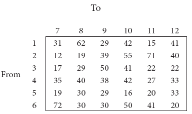
How should the truck be dispersed so as to minimize the total distance travelled?
6.
Evaluate \(\Delta \)\(\left[ \frac { 5x+12 }{ { x }^{ 2 }+5x+6 } \right] \) by taking ‘1’ as the interval of differencing.
7.
A departmental head has four subordinates and four tasks to be performed. The subordinates differ in efficiency and the tasks differ in their intrinsic difficulty. His estimates of the time each man would take to perform each task is given below :
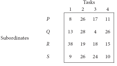
How should the tasks be allocated to subordinates so as to minimize the total man-hours?
8.
Suppose that \({ Q }_{ d }=30-5P+2\frac { dp }{ dt } +\frac { { d }^{ 2 }P }{ { dt }^{ 2 } } \) and Qs = 6 + 3P. Find the equilibrium price for market clearance.
9.
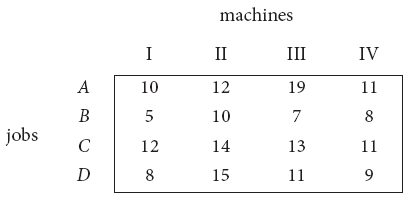
Solve the following assignment problem. Cell values represent cost of assigning job A, B, C and D to the machines I, II, III and IV.
10.
From the following data, calculate the control limits for the mean and range chart.
| Sample No. | 1 | 2 | 3 | 4 | 5 | 6 | 7 | 8 | 9 | 10 |
| Sample Observations | 50 | 51 | 50 | 48 | 46 | 55 | 45 | 50 | 47 | 56 |
| 55 | 50 | 53 | 53 | 50 | 51 | 48 | 56 | 53 | 53 | |
| 52 | 53 | 48 | 50 | 44 | 56 | 53 | 54 | 49 | 55 | |
| 49 | 50 | 52 | 51 | 48 | 47 | 48 | 53 | 52 | 54 | |
| 54 | 46 | 47 | 53 | 47 | 51 | 51 | 57 | 54 | 52 |
11.
Solve the following:
\(\frac { dy }{ dx } \)+ ytan x = cos3 x
12.
In a certain bottling industry the quality control inspector recorded the weight of each of the 5 bottles selected at random during each hour of four hours in the morning.
| Time | Weights in ml | ||||
| 8:00 AM | 43 | 41 | 42 | 43 | 41 |
| 9:00 AM | 40 | 39 | 40 | 39 | 44 |
| 10:00 AM | 42 | 42 | 43 | 38 | 40 |
| 11:00 AM | 39 | 43 | 40 | 39 | 42 |
13.
Ten samples each of size five are drawn at regular intervals from a manufacturing process. The sample means ( \(\overset{-}{X}\) ) and their ranges (R ) are given below:
| Sample number | 1 | 2 | 3 | 4 | 5 | 6 | 7 | 8 | 9 | 10 |
| \(\overset {-}{X}\) | 49 | 45 | 48 | 53 | 39 | 47 | 46 | 39 | 51 | 45 |
| R | 7 | 5 | 7 | 9 | 5 | 8 | 8 | 6 | 7 | 6 |
Calculate the control limits in respect of \(\overset {-}{X}\) chart. (Given A2 = 0.58, D3 = and D4 = 2.115) Comment on the state of control.
14.
Calculate Fisher’s index number to the following data. Also show that it satisfies Time Reversal Test.
| Commodity | Price in Rupees per unit | Number of units | ||
| Price (Rs.) | Quantity (Kg) | Price (Rs.) | Quantity (Kg) | |
| Food | 40 | 12 | 65 | 14 |
| Fuel | 72 | 14 | 78 | 20 |
| Clothing | 36 | 10 | 36 | 15 |
| Wheat | 20 | 6 | 42 | 4 |
| Others | 46 | 8 | 52 | 6 |
15.
Calculate price index number for 2005 by
(a) Laspeyre’s
(b) Paasche’s method
| Commodity | 1995 | 2005 | ||
| Price | Quantity | Price | Quantity | |
| A | 5 | 60 | 15 | 70 |
| B | 4 | 20 | 8 | 35 |
| C | 3 | 15 | 6 | 20 |
16.
Solve the following homogeneous differential equations.
\((x-y)\frac { dy }{ dx } =x+3y\).
17.
The annual production of a commodity is given as follows :
\(\begin{array}{|c|c|} \hline \text { Year } & \text { Production (in tones) } \\ \hline 1995 & 155 \\ \hline 1996 & 162 \\ \hline 1997 & 171 \\ \hline 1998 & 182 \\ \hline 1999 & 158 \\ \hline 2000 & 180 \\ \hline 2001 & 178 \\ \hline \end{array}\)
Fit a straight line trend by the method of least squares.
18.
Solve the differential equation \(\frac { dy }{ dx } =\frac { x-y }{ x+y } \)
19.
Calculate the cost of living index number by consumer price index number for the year 2016 with respect to base year 2011 of the following data
\(\begin{array}{|c|c|c|c|} \hline & {\text { Price }} & \\ \begin{array}{c} \text { Commodities } \\ \text { } \end{array} & \begin{array}{c} \text { Base } \\ \text { year } \end{array} & \begin{array}{c} \text { Current } \\ \text { year } \end{array} & \text { Quantity } \\ \hline \text { Rice } & 32 & 48 & 25 \\ \hline \text { Sugar } & 25 & 42 & 10 \\ \hline \text { Oil } & 54 & 85 & 6 \\ \hline \text { Coffee } & 250 & 460 & 1 \\ \hline \text { Tea } & 175 & 275 & 2 \\ \hline \end{array}\)
20.
Calculate Fisher’s price index number and show that it satisfies both Time Reversal Test and Factor Reversal Test for data given below.
| Commodities | Base Year | Current Year | ||
| Price | Quantity | Price | Quantity | |
| Rice | 10 | 5 | 11 | 6 |
| Wheat | 12 | 6 | 13 | 4 |
| Rent | 14 | 8 | 15 | 7 |
| Fuel | 16 | 9 | 17 | 8 |
| Transport | 18 | 7 | 19 | 5 |
| Miscellaneous | 20 | 4 | 21 | 3 |
21.
Solve 3extan ydx +(1 + ex)sec2ydy = 0 given y(0) = \(\frac { \pi }{ 4 } \)
22.
23.
The mean breaking strength of cables supplied by a manufacturer is 1,800 with a standard deviation 100. By a new technique in the manufacturing process it is claimed that the breaking strength of the cables has increased. In order to test this claim a sample of 50 cables is tested. It is found that the mean breaking strength is 1,850. Can you support the claim at 0.01 level of significance.
24.
Evaluate the following integrals as the limit of the sum:
\(\int _{ 0 }^{ 1 }{ { x }^{ 2 } } dx\)
25.
Evaluate the integral as the limit of a sum: \(\int _{ 1 }^{ 2 }{ (2x+1) } dx\)
26.
A sample of 100 measurements at breaking strength of cotton thread gave a mean of 7.4 and a standard deviation of 1.2 gms. Find 95% confidence limits for the mean breaking strength of cotton thread.
27.
Evaluate \(\int _{ 0 }^{ \frac { \pi }{ 2 } }{ \frac { \sin x }{ \sin x+\cos x } } \) dx
28.
Time taken by a construction company to construct a flyover is a normal variate with mean 400 labour days and standard deviation of 100 labour days. If the company promises to construct the flyover in 450 days or less and agree to pay a penalty of Rs. 10,000 for each labour day spent in excess of 450. What is the probability that
(i) the company pays a penalty of atleast Rs. 2,00,000?
(ii) the company takes at most 500 days to complete the flyover?
29.
An experiment succeeds twice as often as it fails, what is the probability that in next five trials there will be
(i) three successes and
(ii) at least three successes
30.
900 light bulbs with a mean life of 125 days are installed in a new factory. Their length of life is normally distributed with a standard deviation of 18 days. What is the expected number of bulbs expire in less than 95 days?
31.
Evaluate \(\int _{ 2 }^{ 3 }{ \frac { { x }^{ 4 }+1 }{ { x }^{ 2 } } } dx\)
32.
What is the probability that a standard normal variate Z will be
(i) greater than 1.09
(ii) less than -1.65
(iii) lying between -1.00 and 1.96
(iv) lying between 1.25 and 2.75
33.
The probability density function of a continuous random variable X is
\(f(x)=\left\{\begin{array}{l} a+b x^{2}, 0 \leq x \leq 1 \\ 0, \text { otherwise } \end{array}\right.\)
where a and b are some constants. Find
(i) a and b if E(X)\(\frac{3}{5}\)
(ii) Var(X).
34.
Evaluate \(\int\left[\frac{1}{\log x}-\frac{1}{(\log x)^{2}}\right] d x\)
35.
Find the consumer’s surplus and producer’s surplus for the demand function pd = 25 − 3x and supply function ps = 5 + 2x.
36.
Suppose that the time in minutes that a person has to wait at a certain station for a train is found to be a random phenomenon with a probability function specified by the distribution function\(F(x)\begin{cases} 0,\quad \text{for}\quad x<0 \\ \frac { 1 }{ 2 } ,\quad \text{for}\quad 0\le x<1 \\ 0,\quad \text{for}\quad 1\le x<2\quad \\ \frac { 1 }{ 4 } ,\quad \text{for}\quad 2\le x<4 \\ 0,\quad \text{for}\quad x\ge 4 \end{cases}\)
(a) Is the distribution function continuous? If so, give its probability density function?
(b) What is the probability that a person will have to wait
(i) more than 3 minutes,
(ii) less than 3 minutes and
(iii) between 1 and 3 minutes?
37.
A firm’s marginal revenue function is MR = 20e-x/10 \(\left( 1-\frac { x }{ 10 } \right) \). Find the corresponding demand function.
38.
Elasticity of a function \(\frac{Ey}{Ex}\) is given by \(\frac{Ey}{Ex}\) = \(\frac { -7x }{ (1-2x)(2+3x) } \). Find the function when x = 2, y = \(\frac{3}{8}\)
39.
The amount of bread (in hundreds of pounds) x that a certain bakery is able to sell in a day is found to be a numerical valued random phenomenon, with a probability function specified by the probability density function f(x) is given by
\(f(x)=\left\{\begin{array}{l} Ax,for \ 0≤x10 \\ A(20−x),for \ 10 ≤x< 20 \\ 0,\quad \quad \quad otherwise \end{array}\right.\)
(a) Find the value of A.
(b) What is the probability that the number of pounds of bread that will be sold tomorrow is
(i) More than 10 pounds,
(ii) Less than 10 pounds, and
(iii) Between 5 and 15 pounds?
40.
41.
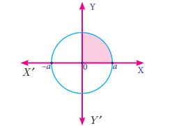
Using integration find the area of the circle whose center is at the origin and the radius is a units.
42.
Find k if the equations x + y + z = 1, 3x − y − z = 4, x+ 5y + 5z = k are inconsistent.
43.
The price of 3 Business Mathematics books, 2 Accountancy books and one Commerce book is Rs. 840. The price of 2 Business Mathematics books, one Accountancy book and one Commerce book is Rs. 570. The price of one Business Mathematics book, one Accountancy book and 2 Commerce books is Rs. 630. Find the cost of each book by using Cramer’s rule.
44.
Find k, if the equations x + y + z = 7, x + 2y + 3z = 18, y + kz = 6 are inconsistent
45.
Evaluate \(\int _{ 1 }^{ 2 }{ \frac { 1 }{ (x+1)(x+2) } } dx\)
46.
Integrate the following with respect x
\(\frac { 3x+2 }{ \left( x-2 \right) \left( x-3 \right) } \)
47.
The subscription department of a magazine sends out a letter to a large mailing list inviting subscriptions for the magazine. Some of the people receiving this letter already subscribe to the magazine while others do not. From this mailing list, 45% of those who already subscribe will subscribe again while 30% of those who do not now subscribe will subscribe. On the last letter, it was found that 40% of those receiving it ordered a subscription. What percent of those receiving the current letter can be expected to order a subscription?
48.
Show that the following system of equations have unique solution:
x + y + z = 3, x + 2y + 3z = 4, x + 4y + 9z = 6 by rank method.
1.
\(\Delta =\left| \begin{matrix} 2 & 1 & -1 \\ 1 & 1 & 1 \\ 1 & -2 & 3 \end{matrix} \right| =2\)
\(\left| \begin{matrix} 1 & 1 \\ -2 & -3 \end{matrix} \right| -1\left| \begin{matrix} 1 & 1 \\ 1 & -3 \end{matrix} \right| -1\left| \begin{matrix} 1 & 1 \\ 1 & -2 \end{matrix} \right| \)
= 2 (-3+2) - 1 (-3 -1) -1 (-2-1)
= 2(-1) -1 (-4) -1 (-3)
= -2 + 4 + 3 = 5.
Since\(\Delta \neq 0\),
we can apply Cramer's rule and the system is consistent with unique solution.
\(x=\left| \begin{matrix} 3 & 1 & -1 \\ 1 & 1 & 1 \\ 4 & -2 & 3 \end{matrix} \right| =3\left| \begin{matrix} 1 & 1 \\ -2 & -3 \end{matrix} \right| -1\left| \begin{matrix} 1 & 1 \\ 4 & -3 \end{matrix} \right| -1\left| \begin{matrix} 1 & 1 \\ 4 & -2 \end{matrix} \right| \)
= 3(-3 + 2) -1(-3 -4) -1(-2 -4)
= 3 (-1) -1 (-7) -1 (-6)
= -3 + 7 + 6 = 10.
\(\Delta y=\left| \begin{matrix} 2 & 3 & -1 \\ 1 & 1 & 1 \\ 1 & 4 & -3 \end{matrix} \right| =2\left| \begin{matrix} 1 & 1 \\ 4 & -3 \end{matrix} \right| -3\left| \begin{matrix} 1 & 1 \\ 1 & -3 \end{matrix} \right| -1\left| \begin{matrix} 1 & 1 \\ 1 & 4 \end{matrix} \right| \)
= 2(-3 -4) -3 (-3 -1) -1 (4-1)
= 2 (-7) -3 (-4) -1(3)
= 14 + 12 - 3 = -5
\(\Delta z=\left| \begin{matrix} 2 & 1 & 3 \\ 1 & 1 & 1 \\ 1 & -2 & 4 \end{matrix} \right| \)
= \(2\left| \begin{matrix} 1 & 1 \\ -2 & 4 \end{matrix} \right| -1\left| \begin{matrix} 1 & 1 \\ 1 & 4 \end{matrix} \right| +3\left| \begin{matrix} 1 & 1 \\ 1 & -2 \end{matrix} \right| \)
= 2(4 + 2) -1(4 -1) + 3(-2 -1)
= 2(6) -1(3) + 3(-3)
= 12 - 3 - 9
= 0
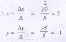
\(z=\cfrac { \Delta z }{ \Delta } =\cfrac { 0 }{ 5 } =0\)
\(\therefore\)Solution set is (2, -1, 0)
2.
Given
| x | -1 | 0 | 1 | 2 |
| y | 202 | 175 | 82 | 55 |
Since we have to find f(0.5) which is at the beginning of the table, use Newton's forward interpolation formula.
xn + nh = 0.5 ⇒ -1 + n(1) = 0.5
⇒ n = 0.5 + 1 = 1.5
∴ y(0.5) = \(\frac { n }{ 1! } { \triangle y }_{ 0 }+\frac { n(n+1) }{ 2! } { \triangle }^{ 2 }{ y }_{ 0 }+\frac { n(n+1)(n+2) }{ 3! } { \triangle }^{ 3 }{ y }_{ 0 }\)
The difference table is
| x | y | Δy | Δ2y | Δ3y |
|---|---|---|---|---|
| -1 | 202 | |||
| 0 | 175 | |||
| 1 | 82 | -93 | -66 | |
| 2 | 55 | -27 | 66 | 132 |
∴ y(0.5) = 202+\(\frac { 1.5 }{ 1! } (-27)+\frac { (1.5)(1.5-1) }{ 2! } (-66)+\frac { (1.5)(1.5-1)(1.5-2) }{ 3! } (132)\)
= 202 - 40.5 + (1.5) (.5) (-33) + \(\frac { (1.5)(.5)(-0.5) }{ 6(132) } \) (132)
= 202 - 40.5 - 24.75 - 8.25
= 202 -73.5
= 128.5
Hence f(0.5) = 128.5
3.
Given
| Year | 1974 | 1978 | 1982 | 1990 |
| Output in 1000 tones | 25 | 60 | 80 | 170 |
Here the intervals are unequal.
∴ By Lagranges interpolation formula, we have
x0 = 1974, x1 = 1978, x2 = 1982, x3 = 1990
y0 = 25, y1 = 60, y2 = 80, y3 = 170 and x = 1986.
∴ y = f(x) = \(\frac { (x-{ x }_{ 1 })(x-{ x }_{ 2 })(x-{ x }_{ 3 }) }{ ({ x }_{ 0 }-{ x }_{ 1 })({ x }_{ 0 }-{ x }_{ 2 })({ x }_{ 0 }-{ x }_{ 3 }) } \times { y }_{ 0 }+\frac { (x-{ x }_{ 0 })(x-{ x }_{ 2 })(x-{ x }_{ 3 }) }{ ({ x }_{ 1 }-{ x }_{ 0 })({ x }_{ 1 }-{ x }_{ 2 })(x_{ 1 }-{ x }_{ 3 }) } \times { y }_{ 1 }+\frac { (x-{ x }_{ 0 })(x-{ x }_{ 1 })(x-{ x }_{ 3 }) }{ ({ x }_{ 2 }-{ x }_{ 0 })({ x }_{ 2 }-{ x }_{ 1 })({ x }_{ 2 }-{ x }_{ 3 }) } \times { y }_{ 2 }+\frac { (x-{ x }_{ 0 })(x-{ x }_{ 1 })(x-{ x }_{ 2 }) }{ ({ x }_{ 3 }-{ x }_{ 0 })({ x }_{ 3 }-{ x }_{ 1 })({ x }_{ 3 }-{ x }_{ 2 }) } \times { y }_{ 3 }\)
\(\frac { (x-{ x }_{ 0 })(x-{ x }_{ 2 })(x-{ x }_{ 3 }) }{ ({ x }_{ 0 }-{ x }_{ 1 })({ x }_{ 0 }-{ x }_{ 2 })({ x }_{ 0 }-{ x }_{ 3 }) } \times25+\frac { (x-{ x }_{ 0 })(x-{ x }_{ 2 })(x-{ x }_{ 3 }) }{ ({ x }_{ 1 }-{ x }_{ 0 })({ x }_{ 1 }-{ x }_{ 2 })(x_{ 1 }-{ x }_{ 3 }) } \times60+\frac { (x-{ x }_{ 0 })(x-{ x }_{ 1 })(x-{ x }_{ 3 }) }{ ({ x }_{ 2 }-{ x }_{ 0 })({ x }_{ 2 }-{ x }_{ 1 })({ x }_{ 2 }-{ x }_{ 3 }) } \times80+\frac { (x-{ x }_{ 0 })(x-{ x }_{ 1 })(x-{ x }_{ 2 }) }{ ({ x }_{ 3 }-{ x }_{ 0 })({ x }_{ 3 }-{ x }_{ 1 })({ x }_{ 3 }-{ x }_{ 2 }) } \times 70+\frac { (1986-1974)(1986-1982)(1986-1990) }{ (1990-1974)(1990-1978)(1990-1982) } \times 170\)
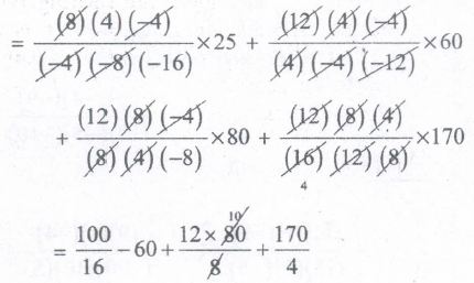
= 6.25 - 60 + 120 + 42.5
y = 108.75
4.
Here the intervals are unequal. By Lagrange’s interpolation formula we have
x0 = 5, x1 = 6, x2 = 9, x3 = 11
y0 = 12, y1 = 13, y2 = 14, y3 = 16
\(y=f(x)=\frac { \left( x-{ x }_{ 1 } \right) \left( x-{ x }_{ 2 } \right) \left( x-{ x }_{ 3 } \right) }{ \left( { x }_{ 0 }-{ x }_{ 1 } \right) \left( x_{ 0 }-{ x }_{ 2 } \right) \left( { x }_{ 0 }-{ x }_{ 3 } \right) } \times { y }_{ 0 }+\frac { \left( x-{ x }_{ 0 } \right) \left( x-{ x }_{ 2 } \right) \left( x-{ x }_{ 3 } \right) }{ \left( { x }_{ 1 }-{ x }_{ 0 } \right) \left( x_{ 1 }-{ x }_{ 2 } \right) \left( { x }_{ 1 }-{ x }_{ 3 } \right) } \times { y }_{ 1 }+\frac { \left( x-{ x }_{ 0 } \right) \left( x-{ x }_{ 2 } \right) \left( x-{ x }_{ 3 } \right) }{ \left( { x }_{ 2 }-{ x }_{ 0 } \right) \left( x_{ 2 }-{ x }_{ 1 } \right) \left( { x }_{ 2 }-{ x }_{ 3 } \right) } \times { y }_{ 2 }+\frac { \left( x-{ x }_{ 0 } \right) \left( x-{ x }_{ 2 } \right) \left( x-{ x }_{ 3 } \right) }{ \left( { x }_{ 3 }-{ x }_{ 0 } \right) \left( x_{ 3 }-{ x }_{ 1 } \right) \left( { x }_{ 3 }-{ x }_{ 2 } \right) } \times { y }_{ 3 }\)
\(=\frac { (x-6)(x-9)(x-11) }{ (5-6)(5-6)(5-11) } (12)+\frac { (x-5)(x-9)(x-11) }{ (6-5)(6-9)(6-9) } (13)+\frac { (x-5)(x-6)(x-11) }{ (9-5)(9-6)(9-11) } (14)+\frac { (x-5)(x-6)(x-9) }{ (11-5)(11-6)(11-9) } (16)\)
Put x = 10
\({ y }_{ (10) }=f\left( 10 \right) =\frac { 4(1)(-1) }{ (-1)(-4)(-6) } (12)+\frac { (5)(1)(-1) }{ (1)(-3)(-5) } (13)+\frac { 5(4)(-1) }{ 4(3)(-2) } (14)+\frac { (5)(4)(1) }{ 6(5)(2) } (16)\)}
= \(\frac { 1 }{ 6 } \left( 12 \right) -\frac { 13 }{ 3 } +\frac { 5\left( 14 \right) }{ 3\times 2 } +\frac { 4\times 16 }{ 12 } \)
= 14.6663
5.
Here the number of rows and columns are equal.
∴ The given assignment problem is balanced.
Step 1: Select a minimum element in each row and subtract this from all the elements in its row.
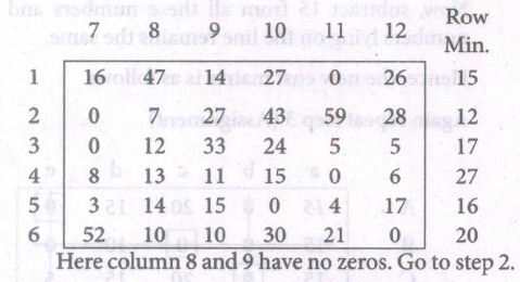
Step 2: Select the minimum element in each column and subtract this from all the elements in its column
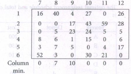
Since each row and column contains atleast one zero, assignments can be made.
Step 3: (Assignment)
Examine the rows with exactly one zero. Mark the zero by and draw a vertical line.
After examining the rows, examine the columns with exactly one zero. Mark the zero by and draw a horizontal line.
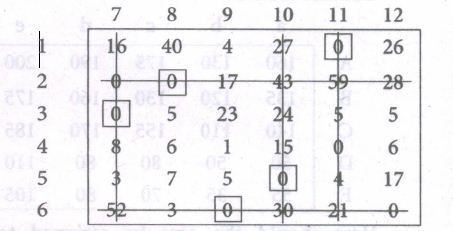
Only 4 assignments are made
Number not lying on the line are
| 40 | 4 | 26 |
| 5 | 23 | 5 |
| 6 | 1 | 6 |
| 7 | 5 | 17 |
and minimum of these numbers are 1.
This number 1 should be subtracted from the above number and 1 should be added to the numbers which are on the intersecting lines (ie. 52,43,59,30,21)and the other numbers remains the same.
A new cost matrix is as follows and repeat step 3.
New cost matrix is
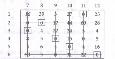
Thus, all the six assignments have been made.
∴ The optimal assignment schedule and total cost is
| Cities From | Cities To | Cost |
| 1 | 11 | 15 |
| 2 | 8 | 19 |
| 3 | 7 | 17 |
| 4 | 9 | 38 |
| 5 | 10 | 16 |
| 6 | 12 | 20 |
| Total Cost | Rs. 125 | |
6.
\(\Delta \)\(\left[ \frac { 5x+12 }{ { x }^{ 2 }+5x+6 } \right] \)
By Partial fraction method
\(\frac { 5x+12 }{ { x }^{ 2 }+5x+6 } =\frac { A }{ x+3 } +\frac { B }{ x+2 } \)
\(A=\frac { 5x+12 }{ x+12 } [x=-3]=\frac { -15+12 }{ -1 } =\frac { -3 }{ -1 } =-3\)
\(B=\frac { 5x+12 }{ x+3 } \)[x = -2] \(=\frac { 2 }{ 1 } =2\)
\(\frac { 5x+12 }{ { x }^{ 2 }+5x+6 } = \left[ \frac { 3 }{ x+3 } +\frac { 2 }{ x+2 } \right] \)
\(\Delta \frac { 5x+12 }{ { x }^{ 2 }+5x+6 } =\Delta \left[ \frac { 3 }{ x+3 } +\frac { 2 }{ x+2 } \right] \)
\(=\left[ \frac { 3 }{ x+1+3 } -\frac { 3 }{ x+3 } \right] +\left\{ \frac { 2 }{ x+1+2 } -\frac { 2 }{ x+2 } \right\} \)
\(=3\left[ \frac { 1 }{ x+4 } -\frac { 1 }{ x+3 } \right] +2\left[ \frac { 1 }{ x+3 } -\frac { 1 }{ x+2 } \right] \)
\(=\left[ \frac { -3 }{ (x+4)(x+3) } -\frac { 2 }{ (x+3)(2+3) } \right] \)
\(=\frac { -5x-14 }{ (x+2)(x+3)(x+4) } \)
7.
Here the number of rows and columns are equal
∴ The given assignment problem is balanced.
Step 1 : Select a minimum element in each row and subtract this from all the elements in its row.
∴ The cost matrix of the given assignment problem is
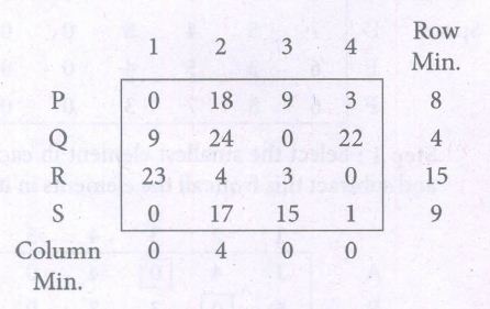
Column 2 has no zero. Go to Step 2.
Step 2 : Select the minimum element in each column and subtract this from all the elements in its column.
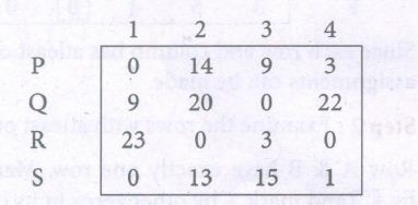
Since each row and column contains atleast one zero, assignments can be made.
Step 3 : Examine the rows with exactly one zero, mark it by and draw a vertical line.
After examining the rows, examine the columns with exactly one zero.
Mark it by and draw a horizontal line.
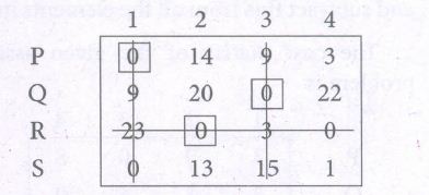
Only 3 assignments have been made.
The numbers not lying on the line are and min. is 1. Subtract 1 from all these numbers and add 1 to 23 which lies on the intersecting lines. Other numbers remain the same.
A new cost matrix is formed and repeat step 3.
∴ The new cost matrix is
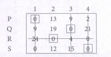
Thus, all the 4 assignments have been made.
∴The optimal assignment schedule and total cost is
| Subordinates | tasks | cost |
|---|---|---|
| P | 1 | 8 |
| Q | 3 | 4 |
| R | 2 | 19 |
| S | 4 | 10 |
| Total Cost | Rs. 41 | |
8.
Given Qd = 30 - 5p + 2\(\frac { dp }{ dt } +\frac { { d }^{ 2 }p }{ dt^{ 1 } } \) and
Qs = -6 + 3p
At equilibrium Qd = Qs
⇒ 30 - 5p+2\(\frac { dp }{ dt } +\frac { { d }^{ 2 }p }{ dt^{ 1 } } \) = -6+3p
⇒ \(\frac { { d }^{ 2 }p }{ dt^{ 2 } } +2\frac { dp }{ dt } \)- 5p + 30 - 6 - p = 0
⇒ \(\frac { { d }^{ 2 }p }{ dt^{ 2 } } +2\frac { dp }{ dt } \)- 8p = 24
The auxiliary equation is m2 + 2m - 8 = 0
⇒ (m + 4) (m - 2) = 0
⇒ m = - 4, 2
∴ C.F. is Ae-4t + Be2t
Particular Integral PI = \(\frac { -24 }{ (D+4)(D-x) } \)e0x
= \(\frac { -24 }{ (0+4)(0-2) } =\frac { -24 }{ -8 } \)=3
∴ y = CF + PI
∴ The general solution is
P = Ae-4t + Be2t + 3.

9.
Here the number of rows and columns are equal.
\(\therefore\)The given assignment problem is balanced.
Now let us find the solution.
Step 1: Select a smallest element in each row and subtract this from all the elements in its row.
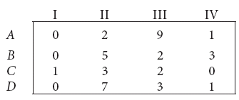
Look for atleast one zero in each row and each column.Otherwise go to step 2.
Step 2 : Select the smallest element in each column and subtract this from all the elements in its column.
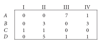
Since each row and column contains atleast one zero, assignments can be made.
Step 3 (Assignment):
Examine the rows with exactly one zero. First three rows contain more than one zero. Go to row D.
There is exactly one zero. Mark that zero by \(\square\) (i.e) job D is assigned to machine
I . Mark other zeros in its column by\(\text { X }\).
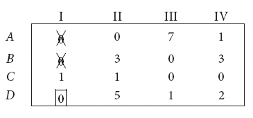
Step 4: Now examine the columns with exactly one zero. Already there is an assignment in column I. Go to the column II. There is exactly one zero. Mark that zero by \(\square\) . Mark other zeros in its row by\(\text { X }\).
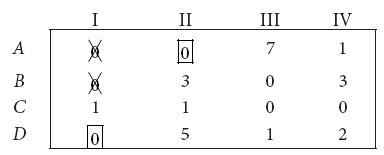
Column III contains more than one zero. Therefore proceed to Column IV, there is exactly one zero. Mark that zero by \(\square\) . Mark other zeros in its row by \(\text { X }\).
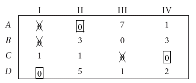
Step 5: Again examine the rows. Row B contains exactly one zero. Mark that zero by \(\square\).
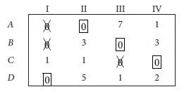
Thus all the four assignments have been made. The optimal assignment schedule and total cost is
\(\begin{array}{|c|c|c|} \hline \text { Job } & \text { Machine } & \text { cost } \\ \hline \text { A } & \text { II } & 12 \\ \hline \text { B } & \text { III } & 7 \\ \hline \text { C } & \text { IV } & 11 \\ \hline \text { D } & \text { I } & 8 \\ \hline {\text { Total cost }} \ && 38 \\ \hline \end{array}\)
The optimal assignment (minimum) cost
= Rs. 38
10.
| Sample No. | Observation | Total | x | R = Xmax - Xmin | ||||
| 1 | 2 | 3 | 4 | 5 | ||||
| 1 | 50 | 55 | 52 | 49 | 54 | 260 | 52 | 55-49 = 6 |
| 2 | 51 | 50 | 53 | 50 | 46 | 250 | 50 | 53-46 = 7 |
| 3 | 50 | 53 | 48 | 52 | 47 | 250 | 50 | 53-47 = 6 |
| 4 | 48 | 53 | 50 | 51 | 53 | 255 | 51 | 53-48 = 5 |
| 5 | 46 | 50 | 44 | 48 | 47 | 235 | 47 | 50-44 = 6 |
| 6 | 55 | 51 | 56 | 47 | 51 | 260 | 52 | 56-47=9 |
| 7 | 45 | 48 | 53 | 48 | 51 | 245 | 49 | 53-45=8 |
| 8 | 50 | 56 | 54 | 53 | 57 | 270 | 54 | 57-50 = 7 |
| 9 | 47 | 53 | 49 | 52 | 54 | 255 | 51 | 54-47 = 7 |
| 10 | 56 | 53 | 55 | 54 | 52 | 270 | 54 | 56-52 = 4 |
| 510 | 65 | |||||||
\(\overline {\overline{X}}\) = \(\frac {510}{10}\) = 51
\(\overline {R}\) = \(\frac {65}{10}\) = 6.5
The control limits of mean chart are
UCL = \(\overline {\overline{X}} + A_{2} \overline{R}\)
= 51 + 0.577 (6.5)
= 51 + 3.75 = 57.75
CL = \(\overline {\overline{X}}\) = 51
LCL = \(\overline {\overline{X}} - A_{2} \overline{R}\)
= 51 - 3.75 = 47.25
The control limits of range chart are
UCL = D4\(\overline {R}\) = 2.114 (6.3) = 13.32
CL = \(\overline {R}\) = 6.5
[For n=5, A2 = 0.577, D3 = 0, D4 = 2.114]
LCL = D3\(\overline {R}\) = 0
11.
The given differential equation is of this form
\(\frac { dy }{ dx } \)+Py=Q where
P = tan x; Q = cos3x
∴ \(\int { p } dx=\int { \tan x } dx\) = log secx
∴ Integrating factor (I.F) = \(e^{ \int { p } dx }\) = elogx secx
= sec x
Hence, the solution is
\(ye^{ \int { p } dx }=\int { Q } .e^{ \int { p } dx }dx+c\)
⇒ y sec x =\(\\ \int { cos^{ 3 }x } \)dx+c
[∴ cos 2x = 2cos2x-1]
⇒ 2 cos2x = 1 + cos2x
⇒ cos2x = \(\frac { 1+cos2x }{ 2 } \)]
⇒ y secx = \(\int { \cos^{ 3 }x.\frac { 1 }{ \cos x } } \)dx+c
⇒y sec x =\(\int { cos^{ 2 }x } dx+c\)
⇒ y sec x =\(\int { \left( \frac { 1+cos2x }{ 2 } \right) } dx+c\)
⇒ y sec x = \(\frac { 1 }{ 2 } \left[ x+\frac { \sin 2x }{ 2 } \right] \)+c
12.
| Time | Weight in ml | Total | \(\overline {X}\) | R = x max - xmin | ||||
| 1 | 2 | 3 | 4 | 5 | ||||
| 8.00 AM | 43 | 41 | 42 | 43 | 41 | 210 | \(\frac {210}{5} = 42\) | 43-41 = 2 |
| 9:00 AM | 40 | 39 | 40 | 39 | 44 | 202 | \(\frac {202}{5} = 40.4\) | 43-41 = 2 |
| 10.00 AM | 42 | 42 | 43 | 38 | 40 | 205 | \(\frac {205}{5} = 41\) | 43-38 = 5 |
| 11:00 AM | 39 | 43 | 40 | 39 | 42 | 203 | \(\frac {203}{5} = 40.6\) | 43-39 = 4 |
| 164 | 16 | |||||||
\(\overline {\overline{X}}\) = \(\frac {164}{4}\) = 41
\(\overline {R}\) = \(\frac {16}{4}\) = 4
Control limits for \(\overline {X}\) - chart
UCL = \(\overline {\overline{X}} + A_{2} \overline {R}\)
= 41 + 0.577 (4)
= 41 + 2.308 = 43.31
CL = \(\overline {\overline{X}} \) = 41
[when n = 5, A2= 0.577, D3 = 0, D4 = 2.114]
LCL = \(\overline {\overline{X}} - A_{2} \overline {R}\)
= 41 - 2.308 = 38.69
The control limits of R-chart are
UCL = D4 \(\overline{R}\) = 2.114 (4) = 8.44
CL = \(\overline{R}\) = 4
LCL = D3 \(\overline{R}=0\)
13.
\(\begin{array}{|c|c|c|c|c|c|c|c|c|c|c|c|} \hline \text { Sample number } & 1 & 2 & 3 & 4 & 5 & 6 & 7 & 8 & 9 & 10 & \text { Total } \\ \hline \bar{X} & 49 & 45 & 48 & 53 & 39 & 47 & 46 & 39 & 51 & 45 & 462 \\ \hline \mathbf{R} & 7 & 5 & 7 & 9 & 5 & 8 & 8 & 6 & 7 & 6 & 68 \\ \hline \end{array}\)
\(\overline{\bar{X}}=\frac{\sum \bar{X}}{10}=\frac{462}{10}=46.2 \)
\(\bar{R}=\frac{\sum R}{10}=\frac{68}{10}=6.8 \)
\(\text { The control limits for } \overline{\mathrm{X}} \text { chart is }\)
\(\mathrm{UCL}=\overline{\overline{\mathrm{X}}}+\mathrm{A}_{2} \overline{\mathrm{R}}=46.2+(0.58)(6.8)=50.14\)
\(\mathrm{CL}=46.2\)
\(\mathrm{LCL}=\overline{\mathrm{X}}-\mathrm{A}_{2} \overline{\mathrm{R}}=46.2-(0.58)(6.8)=42.26 \)
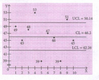
The control limits for range chart is
\(\mathrm{UCL}=\mathrm{D}_{4} \overline{\mathrm{R}}=(2.115)(6.8)=14.38 \)
\(\mathrm{CL}=\overline{\mathrm{R}}=6.8 \)
\(\mathrm{LCL}=\mathrm{D}_{3} \overline{\mathrm{R}}=0(6.8)=0\)
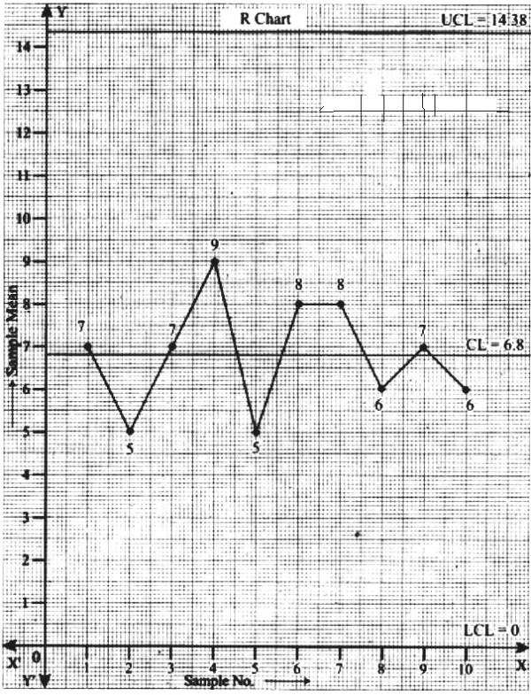
From the \(\overline X\) chart, we see that 4 points are outside the control limit lines. So we say that the process is out of control.
Conclusion: The above diagram shows all the three control lines with the data points plotted, since 2 points fall out of the control limits, we can say that the process is out of control.
14.
| Commodity | 2016 | 2017 | ||
| p0 | q0 | p1 | q1 | |
| Food | 40 | 12 | 65 | 14 |
| Fuel | 72 | 14 | 78 | 20 |
| Clothing | 36 | 10 | 36 | 15 |
| Wheat | 20 | 6 | 42 | 4 |
| Others | 46 | 8 | 52 | 6 |
| p0q0 | p1q1 | p1q0 | p0q1 |
| 480 | 910 | 780 | 560 |
| 1008 | 1560 | 1092 | 1440 |
| 120 | 168 | 252 | 80 |
| 368 | 312 | 416 | 276 |
| 2336 | 3490 | 2900 | 2896 |
Fisher's price index number
\(P^{F}_{01}\) = \(\sqrt \frac {\sum p_{1}q_{0}\times \sum p_{1}q_{1}}{{\sum p_{0}q_{0}\times \sum p_{0}q_{1}}}\) × 100
= \(\sqrt \frac {2900\times3490}{2336\times2896} \times 100\)
= \(\sqrt \frac{10121000}{6765056} \times{100}\)
= \(\sqrt{1.496}\times{100}\)
\(P^{F}_{01}\) = 122.31
Time Reversal Test
P01 × P10 = \(\sqrt \frac {\sum p_{1}q_{0}\times \sum p_{1}q_{1}\times{\sum p_{0}q_{1}\times \sum p_{0}q_{0}}}{{\sum p_{0}q_{0}\times \sum p_{0}q_{1}\times \sum p_{1}q_{1}\times \sum p_{1}q_{0}}}\)
= \(\sqrt \frac {2900\times3490\times{2896\times2336}}{2336\times2896\times3490\times2900}\)
= \(\sqrt {1}\) = 1
Hence, it satisfies time reversal test.
15.
| Commodity | 1995 | 2005 | ||
| Price(p0) | (q0) | Price | Quantity | |
| A | 5 | 60 | 15 | 70 |
| B | 4 | 20 | 8 | 35 |
| C | 3 | 15 | 6 | 20 |
| p0q0 | p0q1 | p1q0 | p1q1 |
| 300 | 350 | 900 | 1050 |
| 80 | 140 | 160 | 280 |
| 45 | 60 | 90 | 120 |
| 425 | 550 | 1150 | 1450 |
Laspeyre's price index number
\(P^{L}_{01}\) = \({\frac {\sum p_{1}q_{0}}{\sum p_{0}q_{0}}} \times 100\)
= \(\frac {1150}{425} \times {100}\) = 270.58
Paasche's index number
\(P^{L}_{01}\) = \({\frac {\sum p_{1}q_{0}}{\sum p_{0}q_{1}}} \times 100\)
= \(\frac {1450}{550} \times {100}\) = 263.63
16.
\(\frac { dy }{ dx } =\frac { x+3y }{ x-y } \)
Since the numerator and denominator are homogeneous functions of degree 1,
put y = vx and \(\frac { dy }{ dx } \) = v + x\(\frac { dv}{ dx } \)
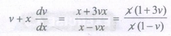
⇒ x\(\frac { dv }{ dx } =\frac { 1+3v }{ 1-v } -v=\frac { 1+3v-v(1-v) }{ 1-v } \)
= \(\frac { 1+3v-v+v^{ 2 } }{ 1-v } \)
⇒ \(x\frac { dv }{ dx } =\frac { 1+2v+v^{ 2 } }{ 1-v } \)
separating the variables we get,
\(\frac { 1-v }{ 1+2v+{ v }^{ 2 } } dv=\frac { dx }{ x } \)
⇒ \(\int { \frac { (1-v)dv }{ { v }^{ 2 }+2v+1 } } =\int { \frac { dx }{ x } } \)
⇒ \(\int { \frac { (1-v)dv }{ (v+1)^{ 2 } } } \) = log x + log c
\(\frac { 1-v }{ (v+1)^{ 2 } } =\frac { A }{ v+1 } +\frac { B }{ (v+1)^{ 2 } } \)
1-v = A(v+1)+B
put v = -1,
2 = B
1 = A + B ⇒ 1 = A+2
⇒ A = -1
∴ \(\frac { 1-v }{ (v+1)^{ 2 } } =\frac { -1 }{ v+1 } +\frac { 2 }{ (v+1) } \)
⇒ \(\int { \frac { -1 }{ v+1 } } dv+\int { \frac { 2 }{ (v+1)^{ 2 } } } dv\) = log xc
⇒ -log (v+1) - \(\frac { 2 }{ v+1 } \) = log xc
⇒ \(\frac { -2 }{ v+1 } \) = log xc + log(v+1)
⇒ \(\frac { -2 }{ v+1 } \) = log xc(v+1)
Replace v by \(\frac{y}{x}\) we get,
\(\frac { -2 }{ \frac { y }{ x } +1 } =logxc\left( \frac { y }{ x } +1 \right) \)
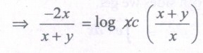
⇒ \(\frac { -2x }{ x+y } \) = logc (x+y)
⇒ e-2x/x+y = c(x+y)
⇒ x+y = \(\frac { 1 }{ c } \) e-2x/x+y
⇒ x+y = ke-2x+x+y where k = \(\frac { 1 }{ c } \).
17.
| Year X | Production in tonnes (Y) | X = x-1998 | X2 | XY |
| 1995 | 155 | -3 | 9 | -465 |
| 1996 | 162 | -2 | 4 | -324 |
| 1997 | 171 | -1 | 1 | -171 |
| 1998 | 182 | 0 | 0 | 0 |
| 1999 | 158 | 1 | 1 | 158 |
| 2000 | 180 | 2 | 4 | 360 |
| 20001 | 178 | 3 | 9 | 534 |
| 1186 | 0 | 28 | 92 |
Since \(\sum\)X = 0, a = \(\frac {\sum Y}{n}\) = \(\frac {1186}{7}\) = 169.428.
b = \(\frac {\sum XY}{\sum X^2}\) \(\frac {92}{28}\) = 3.285
∴ The required equation of the straight line trend is given by Y = a + bX
\(\Rightarrow \) Y= 69.428 + 3.285 (x - 1998)
18.
\(\frac { dy }{ dx } =\frac { x-y }{ x+y } \) ..... (1)
This is a homogeneous differential equation.
Now put y = vx and \(\frac { dy }{ dx } =v+x\frac { dv }{ dx } \)
∴ (1) ⇒ \(v+x\frac { dv }{ dx } =\frac { x-vx }{ x+vx } \)
\(=\frac { 1-v }{ 1+v } \)
\(x\frac { dv }{ dx } =\frac { 1-v }{ 1+v } -v\)
\(=\frac { 1-2v-{ v }^{ 2 } }{ 1+v } \)
\(\frac { 1+v }{ { v }^{ 2 }+2v-1 } dv=\frac { -dx }{ x } \)
Multiply 2 on both sides
\(\frac { 2+v }{ { v }^{ 2 }+2v-1 } dv=-2\frac { -dx }{ x } \)
On Integration
ഽ\(\frac { 2+v }{ { v }^{ 2 }+2v-1 } \)dv = -2ഽ\(\frac { -dx }{ x } \)
log(v2+2v − 1) = −2log x + log c
v2+2v − 1 = \(\frac { c }{ { x }^{ 2 } } \)
x2(v2+2v−1) = c
Now, Replace \(v=\frac { y }{ x } \)
\({ x }^{ 2 }\left[ \frac { { { y }^{ 2 } } }{ { x }^{ 2 } } +\frac { 2y }{ x } -1 \right] =c\)
y2 + 2xy − x2 = c is the solution
19.
Here the base year quantities are given, therefore we can apply Aggregate Expenditure Method.
| Commodities | Price | Quantity (q0) |
p0q0 | p1q0 | |
| Base year (P0) | Current year (P1) | ||||
| Rice | 32 | 48 | 25 | 800 | 1200 |
| Sugar | 25 | 42 | 10 | 250 | 420 |
| Oil | 54 | 85 | 6 | 324 | 510 |
| Coffe | 250 | 460 | 1 | 250 | 460 |
| Tea | 175 | 275 | 2 | 350 | 550 |
| Total | 1974 | 3140 | |||
Cost of Living Index Number=\(\frac { \sum { { p }_{ 1 }{ q }_{ 0 } } }{ \sum { { p }_{ 0 }{ q }_{ 0 } } } \times 100=\frac { 3140 }{ 1974 } \times 100 = 159.0679\)
Hence, the Cost of Living Index Number for a particular class of people for the year 2016 is increased by 59.0679 % as compared to the year 2011.
20.
| Commodities | Base Year | Current Year | p0q0 | p0q1 | p1q0 | p1q1 | ||
| Price (p0) |
Quantity (q1) |
Price ((p0)) |
Quantity (q1) |
|||||
| Rice | 10 | 5 | 11 | 6 | 50 | 60 | 55 | 66 |
| Wheat | 12 | 6 | 13 | 4 | 72 | 48 | 78 | 52 |
| Rent | 14 | 8 | 15 | 7 | 112 | 98 | 120 | 105 |
| Fuel | 16 | 9 | 17 | 8 | 144 | 128 | 153 | 136 |
| Transport | 18 | 7 | 19 | 5 | 126 | 90 | 133 | 95 |
| Miscellaneous | 20 | 4 | 21 | 3 | 80 | 60 | 84 | 63 |
| Total | 584 | 484 | 623 | 517 | ||||
Fisher’s price index number
\({ P }_{ 01 }^{ F }=\left( \sqrt { \frac { \sum { { p }_{ 1 }{ q }_{ 10 } } \times \sum { { p }_{ 1 }{ q }_{ 1 } } }{ \sum { { p }_{ 0 }{ q }_{ 0 } } \times \sum { { p }_{ 0 }{ q }_{ 1 } } } } \right) \times 100=\left( \sqrt { \frac { 623\times 517 }{ 584\times 484 } } \right) \times 100=106.74\)
Time Reversal Test: P01 × P10 = 1
\({ P }_{ 01 }\times { P }_{ 10 }=\sqrt { \left( \frac { \sum { { p }_{ 1 }{ q }_{ 0 } } \times \sum { { p }_{ 1 }{ q }_{ 1 } } \times \sum { { p }_{ 0 }{ q }_{ 1 } } \times \sum { { p }_{ 0 }{ q }_{ 0 } } }{ \sum { { p }_{ 0 }{ q }_{ 0 } } \times \sum { { p }_{ 0 }{ q }_{ 1 } } \times \sum { { p }_{ 1 }{ q }_{ 1 } } \times \sum { { p }_{ 1 }{ q }_{ 0 } } } \right) } \)
\({ P }_{ 01 }\times { P }_{ 10 }=\sqrt { \left( \frac { 623\times 517\times 484\times 584 }{ 584\times 487\times 517\times 623 } \right) } \)
P01 x P10 = 1
Factor Reversal Test
\({ P }_{ 01 }\times { Q }_{ 01 }=\frac { \sum { { p }_{ 1 }{ q }_{ 1 } } }{ \sum { { p }_{ 0 }{ q }_{ 0 } } } \)
\({ P }_{ 01 }\times { P }_{ 01 }=\sqrt { \left( \frac { \sum { { p }_{ 1 }{ q }_{ 0 } } \times \sum { { p }_{ 1 }{ q }_{ 1 } } \times \sum { { p }_{ 1 }{ q }_{ 0 } } \times \sum { { p }_{ 1 }{ q }_{ 1 } } }{ \sum { { p }_{ 0 }{ q }_{ 0 } } \times \sum { { p }_{ 0 }{ q }_{ 1 } } \times \sum { { p }_{ 0 }{ q }_{ 0 } } \times \sum { { p }_{ 0 }{ q }_{ 1 } } } \right) } \)
\({ P }_{ 01 }\times { P }_{ 10 }=\sqrt { \left( \frac { 623\times 517\times 484\times 517 }{ 584\times 484\times 584\times 623 } \right) } \)
\({ P }_{ 01 }\times { P }_{ 01 }=\sqrt { \left( \frac { 517\times 517 }{ 585\times 584 } \right) } =\frac { 517 }{ 584 } \)
\({ P }_{ 01 }\times { P }_{ 01 }=\frac { \sum { { p }_{ 1 }{ q }_{ 1 } } }{ \sum { { p }_{ 0 }{ q }_{ 0 } } } \)
21.
Given 3ex tan y dx + (1 + ex)sec2y dy = 0
3ex tan y dx = −(1 + ex)sec2 y dy
\(\frac { { 3e }^{ x } }{ 1+{ e }^{ x } } dx=-\frac { { sec }^{ 2 }y }{ tany } dy\)
Integrating, we get 3ഽ\(\frac { { 3e }^{ x } }{ 1+{ e }^{ x } } dx\) = -ഽ\(\frac { { sec }^{ 2 }y }{ tany } dy\) + c
3log(1+ ex ) = −log tan y + log c \(\left[ \therefore \int { \frac { f'(x) }{ f(x) } dx=logf(x) } \right] \)
log(1+ex)3 + log tan y = log c
log [(1 + ex)3 tan y ] = log c
(1+ex)3 tan y = c (1)
Given y(0) = \(\frac { \pi }{ 4 } \) (i.e) y = \(\frac { \pi }{ 4 } \) at x =0
(1) ⇒ (1 +e0 )3 tan \(\frac { \pi }{ 4 } \) = c
23 (1) = c
⇒ c = 8
Hence the required solution is (1 +ex)3 tan y = 8
22.
23.
Sample size n = 50,
Sample mean \(\bar { X } \) = 1850
Population mean μ = 1800
Population standard deviation σ = 100
Null Hypotheses H0:
μ = 1800 (i.e., To claim that the breaking strength of the cables have increased)
Alternative Hypotheses H1:
μ≠1800(To claim that the breaking strength of the cables have not increased)
The level of significance ∝ = 1% =.001
Applying the test statistic,
\(Z=\frac { \bar { X } -\mu }{ \frac { \sigma }{ \sqrt { n } } } \)
\(\Rightarrow Z=\frac { 1850-1800 }{ \frac { 100 }{ \sqrt { 50 } } } =\frac { 50 }{ \frac { 100 }{ 7.07 } } =\frac { 50 }{ 14.144 } =3.535\)
\(\Rightarrow \therefore Z=3.535\)
The Significant value \({ Z }_{ \frac { \alpha }{ 2 } }=2.58\)
Here \(Z<{ Z }_{ \frac { \alpha }{ 2 } }i.e.,3.535<2.58\)
Inference: Since \(Z<{ Z }_{ \frac { \alpha }{ 2 } }\) at 1% level of significance, the null hypothesis Ho is rejected.
Hence, we conclude that μ≠ 1800 and we cannot support the claim that the breaking strength of the cables have increased.
24.
\(\int _{ a }^{ b }{ f(x)dx } =\underset { n\rightarrow \infty \\ h\rightarrow 0 }{ lim } \sum _{ r=1 }^{ n }{ h.f\left( a+rh \right) } \)
Here a = 0, b = 1
\(h=\cfrac { b-a }{ n } =\cfrac { 1-0 }{ n } =\cfrac { 1 }{ n } \)
and f(x) = x2
Now, \(f(a+rh)=f\left( 0+r.\cfrac { 1 }{ n } \right) =f\left( \cfrac { r }{ n } \right) \)
= \(\left( \cfrac { r }{ n } \right) ^{ 2 }=\cfrac { { r }^{ 2 } }{ { n }^{ 2 } } \)
\(\therefore \int _{ 0 }^{ 1 }{ { x }^{ 2 }dx } =\underset { n\rightarrow \infty }{ lim } \sum _{ r=1 }^{ n }{ \frac { 1 }{ n } } \left( \frac { { r }^{ 2 } }{ { n }^{ 2 } } \right) \)
= \(\underset { n\rightarrow \infty }{ lim } \frac { 1 }{ { n }^{ 3 } } .\frac { n(n+1)(2n+1) }{ 6 } \)
\(\left[ \therefore \sum _{ r=1 }^{ n }{ { r }^{ 2 }=\cfrac { n(n+1)(2n+1) }{ 6 } } \right] \)
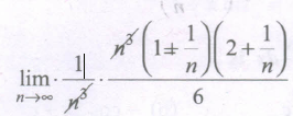
[Taking n common from each bracket]
= \(\cfrac { 1 }{ 6 } .\underset { n\rightarrow \infty }{ lim } \left( 1+\cfrac { 1 }{ n } \right) \left( 2+\cfrac { 1 }{ n } \right) \)
= \(\cfrac { 1 }{ 6 } \left( 1+0 \right) \left( 2+0 \right) \)

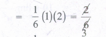
= \(\cfrac { 1 }{ 3 } \)
25.
\(\int _{ a }^{ b }{ f(x) } =\lim _{ n\rightarrow \infty \\ h\rightarrow 0 }{ \sum _{ r=1 }^{ n }{ h } f(a+rh) } \)
Here a = 1, b = 2, \(h=\frac { b-a }{ n } =\frac { 2-1 }{ n } =\frac { 1 }{ n } \) and f(x) = 2x + 1
f (a + rh) = f\(\left( 1+\frac { r }{ n } \right) \)
= \(2\left( 1+\frac { r }{ n } \right) +1\)
= \(2+\frac { 2r }{ n } +1\)
f (a + rh) = 3 + \(\frac {2r }{ n } \)
\(\int _{ 1 }^{ 2 }{ (x) } dx=\lim _{ n\rightarrow \infty }{ \sum _{ r=1 }^{ n }{ \frac { 1 }{ n } \left( 3+\frac { 2r }{ n } \right) } } \)
\(=\lim _{ n\rightarrow \infty }{ \sum _{ r=1 }^{ n }{ \frac { }{ } \left( \frac{3}{n}+\frac { 2r }{ n } \right) } } \)
=\(\overset { lt }{ n\rightarrow \infty } \left[ \frac { 3 }{ n } \sum _{ r=1 }^{ n }{ 1 } +\frac { 2 }{ { n }^{ 2 } } \sum _{ r=1 }^{ n }{ r } \right] \)
= \(\lim _{ n\leftarrow \infty }{ \left[ \frac { 3 }{ n } n+\frac { 2 }{ { n }^{ 2 } } \frac { n(n+1) }{ 2 } \right] } \)
= \(3+\lim _{ n\rightarrow \infty }{ \left( 1+\frac { 1 }{ n } \right) } \)
\(\int _{ 1 }^{ 2 }{ f(x) } dx\) = 3 +1 = 4
26.
Given, sample size = 100, \(\bar x\) = 7.4, since σ is unknown but s = 1.2 is known.
In this problem, we consider \(\breve { \sigma } =s\quad { Z }_{ \frac { \alpha }{ 2 } }=1.96\)
\(S.E=\frac { \breve { \sigma } }{ \sqrt { n } } =\frac { s }{ \sqrt { n } } =\frac { 1.2 }{ \sqrt { 100 } } =0.12\)
Hence 95% confidence limits for the population mean are
\(\bar { x } -{ Z }_{ \frac { \alpha }{ 2 } }\frac { \sigma }{ \sqrt { n } } <\mu <\bar { x } +{ Z }_{ \frac { \alpha }{ 2 } }\frac { \sigma }{ \sqrt { n } } \)
\(7.4-(1.96\times 0.12)\le \mu \le 7.4+(1.96\times 0.12)\)
\(7.4-0.2352\le \mu \le 7.4+0.2352\)
\(7.165\le \mu \le 7.635\)
This implies that the probability that the true value of the population mean breaking strength of the cotton threads will fall in this interval (7.165,7.635) at 95%.
27.
Let I = \(\int _{ 0 }^{ \frac { \pi }{ 2 } }{ \frac { \sin x }{ \sin x+ \cos x } } \)dx .......(1)
I = \(\int _{ 0 }^{ \frac { \pi }{ 2 } }{ \frac { \sin\left( \frac { \pi }{ 2 } -x \right) }{ \sin\left( \frac { \pi }{ 2 } -x \right) +\cos\left( \frac { \pi }{ 2 } -x \right) } } \) dx \(\left[∵ \int _{ 0 }^{ a }{ f(x) } dx=\int _{ 0 }^{ a }{ f(a-x)dx } \right] \)
\(\int _{ 0 }^{ \frac { \pi }{ 2 } }{ \frac { \cos x }{ \cos x+\sin x } } \)dx ....(2)
(1) + (2) ⇒
\(2I=\int _{ \frac { \pi }{ 2 } }^{ \frac { \pi }{ 2 } }{ \left[ \frac { \sin x }{ \sin x+\cos x } +\frac { \cos x }{ \cos x+ \sin x } \right] } \)dx
\(=\int _{ 0 }^{ \frac { \pi }{ 2 } }{ dx } ={ [x] }_{ 0 }^{ \frac { \pi }{ 2 } }=\frac { \pi }{ 2 } \)
\(\therefore I=\frac { \pi }{ 4 } \)
28.
Given μ = 400, σ = 100
(i) Company pays a penalty of atleast Rs. 2,00,000
Penalty per day = Rs.10,000
Number of days = \(\frac { 2,00,000 }{ 10,000 } \) = 20
Hence, the company has taken excess of 20 days
∴ P(atleast 470 days) [∵ 450 + 20 = 470]
= P(X ≥ 470)
When X = 470, Z = \(\frac { X-\mu }{ \sigma } \)
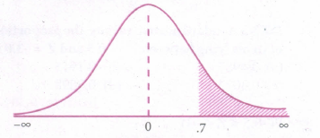
= \(\frac { 470-400 }{ 100 } =\frac { 70 }{ 100 } \) = 0.7
∴ P(X ≥ 470) = P(Z ≥ 0.7)
= P(0.7
P(X ≥ 470) = 0.2420
(ii) P (atmost 500 days) = P(X≤500)
When X = 500, Z = \(\frac { X-\mu }{ \sigma } \)
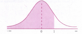
= \(\frac { 500-400 }{ 100 } =\frac { 100 }{ 100 } \)=1
∴ P(X ≤ 500) = P(Z≤1)
= P(-∞
= 0.8413
P(X ≤ 500) = 0.8413
29.
Let p be the probability of success and q be the probability of failure.
Given p = 2q
p = 2(1-p) [∵ p + q = 1]
p = 2-2p ⇒ 3p = 2
p = \(\frac{2}{3}\)
∴ q = 1-p = 1-\(\frac{2}{3}\) = \(\frac{1}{3}\) and n = 5
(i) P (3 successes) = P(X = 3)
= 5C3 \(\left( \frac { 2 }{ 3 } \right) ^{ 3 }\left( \frac { 1 }{ 3 } \right) ^{ 2 }\) ∵ p(x) = nCx pxqn-x, n = 5, x = 3
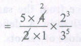
=\(\frac { 10\times 8 }{ 243 } =\frac { 80 }{ 243 } \)
(ii) P (atleast 3 successes)
= P(X ≥ 3)
= 1-P(X < 3)
= 1 - [P(X = 0) + P(X = 1) + P(X = 2)]
= 1-[5C0\(\left( \frac { 2 }{ 3 } \right) ^{ 0 }\left( \frac { 1 }{ 3 } \right) ^{ 5 }\) + 5C1\(\left( \frac { 2 }{ 3 } \right) ^{ 1 }\left( \frac { 1 }{ 3 } \right) ^{ 4 }\) + 5C2\(\left( \frac { 2 }{ 3 } \right) ^{ 2 }\left( \frac { 1 }{ 3 } \right) ^{ 3 }\)]
= 1-\(\left[ \left( \frac { 1 }{ 3 } \right) ^{ 5 }+5\left( \frac { 2 }{ 3 } \right) \left( \frac { 1 }{ { 3 }^{ 4 } } \right) +10\left( \frac { { 2 }^{ 2 } }{ { 3 }^{ 2 } } \right) \left( \frac { 1 }{ { 3 }^{ 3 } } \right) \right] \)
= 1-\(\frac { 1 }{ { 3 }^{ 5 } } \)(1+10+40) = \(1-\frac { 1 }{ 243 } \)(51)
= \(\frac { 243-51 }{ 243 } =\frac { 192 }{ 243 } \).
30.
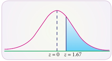
Let X be the normal variate of life of light bulbs with mean 125 and standard deviation 18.
(i) less than 95 days
When X = 95
\(Z=\frac{X-\mu}{\sigma}=\frac{95-125}{18}=-1.667\)
\(P(X<95)=P(Z<-1.667)\)
= 0.5 – P(0 < Z < 1.67)
= 0.5 – 0.4525
= 0.0475
No. of bulbs expected to expire in less than 95 days out of 900 bulbs 900 × .0475 = 43 bulbs
31.
\(\int _{ 2 }^{ 3 }{ \frac { { x }^{ 4 }+1 }{ { x }^{ 2 } } } dx=\int _{ 2 }^{ 3 }{ ({ x }^{ 2 }+{ x }^{ -2 }) } dx\)
= \({ \left[ \frac { { x }^{ 3 } }{ 3 } -\frac { 1 }{ x } \right] }_{ 2 }^{ 3 }\)
= \(\left( 9-\frac { 1 }{ 3 } \right) -\left( \frac { 8 }{ 3 } -\frac { 1 }{ 2 } \right) =\frac { 13 }{ 2 } \)
32.
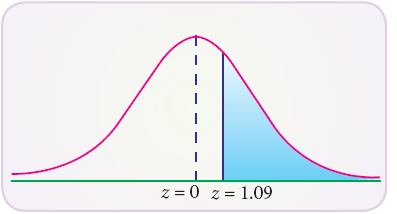
(i) greater than 1.09
The total area under the curve is equal to 1 , so that the total area to the right Z = 0 is 0.5 (since the curve is symmetrical). The area between Z = 0 and 1.09 (from tables) is 0.3621
P(Z > 1.09) = 0.5000 - 0.3621 = 0.1379
The shaded area to the right of Z = 1.09 is the probability that Z will be greater than 1.09
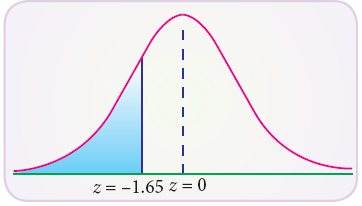
(ii) less than –1.65
The area between -1.65 and 0 is the same as area between 0 and 1.65. In the table the area between zero and 1.65 is 0.4505 (from the table). Since the area to the left of zero is 0.5 , P(Z< 1.65) = 0.5000 – 0.4505 = 0.0495.
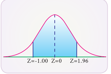
(iii) lying between -1.00 and 1.96
The probability that the random variable Z in between -1.00 and 1.96 is found by adding the corresponding areas :
Area between -1.00 and 1.96 = area between (-1.00 and 0) + area betwn (0 and 1.96)
P(–1.00 < Z < 1.96) = P(–1.00 < Z < 0) + P(0 < Z < 1.96)
= 0.3413 + 0.4750 (by tables)
= 0.8163
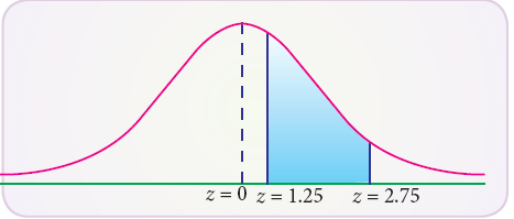
(iv) lying between 1.25 and 2.75
Area between Z = 1.25 and 2.75 = area betwn (z = 0 and z = 2.75)
– area betwn (z=0 and z = 1.25)
P(1.25 < Z < 2.75) = P(0 < Z < 2.75) – P(0 < Z < 1.25)
= 0.4970 - 0.3944 = 0.1026
33.
Given p.d.f is = \(f(x)=\left\{\begin{array}{l} a+b x^{2}, 0 \leq x \leq 1 \\ 0, \text { otherwise } \end{array}\right.\)
Since f(x) is a p.d.f.\(\\ \int _{ -\infty }^{ \infty }{ f(x)dx=1 } \)
\(\Rightarrow \int _{ 0 }^{ 1 }{ (a+{ bx }^{ 2 })dx=1 } \)
\(\Rightarrow { \left[ ax+\frac { { bx }^{ 3 } }{ 3 } \right] }_{ 0 }^{ 1 }=1\Rightarrow a+\frac { b }{ 3 } =1\)
3a+b = 3 [multiplied by 3] ...(1)
Also it is given that E(X) = \(\frac{3}{5}\)
\(\Rightarrow \int _{ 0 }^{ 1 }{ x.f(x)dx=\frac { 3 }{ 5 } } \)
\(\Rightarrow \int _{ 0 }^{ 1 }{ (a+{ bx }^{ 2 })dx=\frac { 3 }{ 5 } } \)
\(\Rightarrow \int _{ 0 }^{ 1 }{ (ax+{ bx }^{ 3 })dx=\frac { 3 }{ 5 } } \)
\(\Rightarrow { \left[ \frac { { ax }^{ 2 } }{ 2 } +\frac { { bx }^{ 4 } }{ 4 } \right] }_{ 0 }^{ 1 }=\frac { 3 }{ 5 } \Rightarrow \frac { a }{ 2 } +\frac { b }{ 4 } =\frac { 3 }{ 5 } \)
\(\Rightarrow 2a+b=\frac { 12 }{ 5 } \) [Multiplies by 4] ...(2)
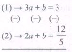
\(a=3-\frac { 12 }{ 5 } =\frac { 15-12 }{ 5 } =\frac { 3 }{ 5 } \)
Substituting a=\(\frac{3}{5}\) in(2) we get,
\(2(\frac { 3 }{ 5 } )+b=\frac { 12 }{ 5 } \Rightarrow \frac { 6 }{ 5 } +b=\frac { 12 }{ 5 } \)
\(\Rightarrow b=\frac { 12 }{ 5 } -\frac { 6 }{ 5 } =\frac { 6 }{ 5 } \)
\(\therefore a=\frac { 3 }{ 5 } ,b=\frac { 6 }{ 5 } \)
ii) \(E({ X }^{ 2 })=\int _{ 0 }^{ 1 }{ { x }^{ 2 }f(x)dx=\int _{ 0 }^{ 1 }{ { x }^{ 2 }\left( \frac { 3 }{ 5 } +\frac { 6 }{ 5 } { x }^{ 2 } \right) dx } } \)
\(\left[ \because a=\frac { 3 }{ 5 } ,b=\frac { 6 }{ 5 } \right] \)
\(=\int _{ 0 }^{ 1 }{ \left( \frac { 3 }{ 5 } { x }^{ 2 }+\frac { 6 }{ 5 } { x }^{ 4 } \right) dx } \)
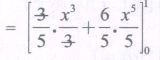
\(=\frac { 1 }{ 5 } (1-0)+\frac { 6 }{ 25 } (1-0)\)
\(=\frac { 1 }{ 5 } +\frac { 6 }{ 25 } =\frac { 5+6 }{ 25 } =\frac { 11 }{ 25 } \)
\(\therefore\) Var (X) = E(X2)-[E(X)]2
\(=\frac { 11 }{ 25 } -{ \left( \frac { 3 }{ 5 } \right) }^{ 2 }\)
\(=\frac { 11 }{ 25 } -\frac { 9 }{ 25 } =\frac { 2 }{ 25 } \)
\(\therefore\) Var (X) =\(\frac{2}{25}\)
34.
ഽ\(\left[ \frac { 1 }{ \log x } -\frac { 1 }{ { \left( \log x \right) }^{ 2 } } \right] dx\) = ഽ\(\left[ \frac { 1 }{ z } -\frac { 1 }{ { z }^{ 2 } } \right] { e }^{ z }dx\)
= ഽ ex [ f(z) +f'(z)] dx
= ez f(z) + c
= ez \(\left[ \frac { 1 }{ z } \right] \) + c
= \(\frac { x }{ \log\ x } \) + c
| Take z = log x ஃdz = \(\frac { 1 }{ x } \)dx ⇒ dx ex dz [∵ x = ex ] and f(z) = \(\frac { 1 }{ z } \) ஃ f'|(z) = \(-\frac { 1 }{ { z }^{ 2 } } \) |
35.
Given demand function Pd = 25 - 3x and
Supply function Ps= 5 + 2x
At market equilibrium, Pd = Ps
⇒ 25-3x = 5+2x
⇒ 25-5 = 2x+3x
⇒ 20 = 5x
⇒ x = \(\frac{20}{5}\)
⇒ x0 = 4
When x0 = 4, p0 = 25-3(4)
= 25-12 = 13
p0 = 13
∴p0x0 = 13(4) = 52
∴ Consumer's surplus
\(CS=\int _{ 0 }^{ x }{ f(x) } dx-{ p }_{ 0 }{ x }_{ 0 }\)
\(\\ =\int _{ 0 }^{ 4 }{ (25-3x)dx-52 } \)
\(={ \left[ 25x-\frac { { 3x }^{ 2 } }{ 2 } \right] }_{ 0 }^{ 4 }-52\)
\(=25(4)-\frac { 3\left( { 4 }^{ 2 } \right) }{ 2 } -52\)
=100-24-52
=100-76
C.S = 24 units
Producer's Surplus
\((PS)={ p }_{ 0 }{ x }_{ 0 }-\int _{ 0 }^{ x }{ g(x)dx } \)
\(=52-\int _{ 0 }^{ 4 }{ (5+2x)dx } \)
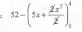
= 52 - (5(4) + 42}
= 52 - (20 + 16)
= 52 - 36
PS = 16 units
36.
Given probability distribution function
\(F(x)\begin{cases} 0,\quad \text{for}\quad x<0 \\ \frac { 1 }{ 2 } ,\quad \text{for}\quad 0\le x<1 \\ 0,\quad \text{for}\quad 1\le x<2\quad \\ \frac { 1 }{ 4 } ,\quad \text{for}\quad 2\le x<4 \\ 0,\quad \text{for}\quad x\ge 4 \end{cases}\)
a) The distribution function F(x) is continuous since it is a step function
We know f'(x) = f(x)
∴ Probability density function
\(F(x)\begin{cases} 0,\quad \text{for}\quad x\le 0 \\ \frac { 1 }{ 2 } ,\quad \text{for}\quad 0\le x<1 \\ 0,\quad \text{for}\quad 1\le x<2\quad \\ \frac { 1 }{ 4 } ,\quad \text{for}\quad 2\le x<4 \\ 0,\quad \text{for}\quad x\ge 4 \end{cases}...(1)\)
(b) (i) Probability that a person will have to wait more than 3 minutes is P(X > 3)
∴ P(X>3) = P(3≤X<4)+P(X≥4)
\(\frac{1}{4}+0=\frac{1}{4}\) [from (1)]
ii) Probability that a person will have to wait less than 3 minutes is P(X < 3)
∴ P(X<3) = P(X≤0)+P(0≤x≤1)+P(1≤x≤2)+P(2≤x≤3)
0 + \(\frac{1}{2}+0+\frac{1}{4}\)[from (1)]
∴ P(X<3) = \(\frac{3}{4}\)
= P(1≤X<2)+P(2≤X<3)
= 0 +\(\frac{1}{4}=\frac{1}{4}\) [from (1)]
37.
Given marginal revenue function.
\(MR=\frac { DR }{ dx } =20{ e }^{ \frac { -x }{ 10 } }\left( 1-\frac { x }{ 10 } \right) \)
\(dR={ 20e }^{ \frac { -x }{ 10 } }\left( 1-\frac { x }{ 10 } \right) dx\)
\(R=\int { { 20e }^{ \frac { -x }{ 10 } } } \left( 1-\frac { x }{ 10 } \right) dx\)
We know that \(\int { { e }^{ ax }[af(x)+f'(x)]dx={ e }^{ ax }f(x) } +c\)
Here \(\\ a=\frac { -1 }{ 10 } ,f(x)=x,\quad f'(x)=1\)
\(R=20\int { { e }^{ \frac { -x }{ 10 } } } \left[ -\frac { 1 }{ 10 } x+1 \right] dx=20{ e }^{ \frac { -x }{ 10 } }x+k\)
\(\Rightarrow R=20{ e }^{ \frac { -x }{ 10 } }x+k\quad ...(1)\)
When x = 0, R = 0
0 = 0 + k ⇒ k = 0
(1) becomes
\(R=20x{ e }^{ \frac { -x }{ 10 } }\)
Demand function P
\(=\frac { R }{ x } =\frac { 20x{ e }^{ \frac { -x }{ 10 } } }{ x } \)
\(\Rightarrow P=20{ e }^{ \frac { -x }{ 10 } }\)
38.
\(\frac { EY }{ Ex } =\frac { -7x }{ (1-2x)(2+3x) } \)
\(\frac { 7 }{ (2x-1)(3x+2) } =\frac { A }{ 2x-1 } +\frac { B }{ 3x+2 } \)
7 = A(3x+2)+B(2x-1)
\(Put\ x=\frac { -2 }{ 3 } 7=B\left( \frac { -4 }{ 3 } -1 \right) 7=B\left( \frac { -7 }{ 3 } \right) \)
\(Put\ x=\frac { 1 }{ 2 } 7=A\left( \frac { 3 }{ 2 } +2 \right) \Rightarrow 7=A\left( \frac { 7 }{ 2 } \right) \)
\(\therefore \frac { 7 }{ (2x-1)(3x+2) } =\frac { 2 }{ 2x-1 } -\frac { 3 }{ 3x+2 } \)
Also, it is given that x = 2, when y \(=\frac{3}{8}\)
\(\Rightarrow \frac { x }{ y } \frac { dy }{ dx } =\frac { -7x }{ (1-2x)(2+3x) } \)

\(=\frac { -7dx }{ (1-2x)(2+3x) } \)
\(\Rightarrow \frac { dy }{ y } =\frac { 7dx }{ (2x+1)(3x+2) } \)
\(\int { \frac { dy }{ y } =\int { \frac { 7dx }{ (2x-)(3x+2) } } } \)
\(\int { \frac { dy }{ y } =\int { \left( \frac { 2 }{ 2x-1 } -\frac { 3 }{ 3x+2 } \right) dx } } \)
\(log\quad y=2\int { \frac { 1 }{ 2x-1 } dx-3\int { \frac { dx }{ 3x+2 } } } \)
\(=2\frac { log|2x-1| }{ 2 } -3\frac { log|3x+2| }{ 3 } +logc\)
\(=log\quad y-log\quad c=log\left| \frac { 2x-1 }{ 3x+2 } \right| \)
\(\Rightarrow log\left| \left( \frac { y }{ c } \right) \right| =log\left| \frac { 2x-1 }{ 3x+2 } \right| \)
\(\Rightarrow \frac { y }{ c } =\frac { 2x-1 }{ 3x+2 } y=c\left( \frac { 2x-1 }{ 3x+2 } \right) \) ....(1)
When \(x=2,y=\frac { 3 }{ 8 } \)
\(\Rightarrow \frac { 3 }{ 8 } =c\left( \frac { 4-1 }{ 8 } \right) \)
\(\frac { 3 }{ 8 } =c\left( \frac { 3 }{ 8 } \right) =c=1\)
\(y=\left( \frac { 2x-1 }{ 3x+2 } \right) \)
\(\Rightarrow y= \frac { 2x-1 }{ 3x+2 }\)
39.
(a) We know that
\(\int _{ -\infty }^{ \infty }{ f(x) } dx=1\)
\(\int _{ 0 }^{ 10 }{ Axdx } +\int _{ 10 }^{ 20 }{ A(20-x)dx=1 } \)
\(A\left\{ { \left[ \frac { { x }^{ 2 } }{ 2 } \right] }_{ 0 }^{ 10 }+{ \left[ 20x-\frac { { x }^{ 2 } }{ 2 } \right] }_{ 10 }^{ 20 } \right\} =1\)
A[(50-0)+(400-200)-(200-50)] = 1
\(A=\frac{1}{100}\)
(b) (i) The probability that the number of pounds of bread that will be sold tomorrow is more than 10 pounds is given by
\(P(10\le X\le 20)=\int _{ 10 }^{ 20 }{ \frac { 1 }{ 100 } (20-x) } dx\)
\(=\frac { 1 }{ 100 } { \left[ 20x-\frac { { x }^{ 2 } }{ 2 } \right] }_{ 10 }^{ 20 }\)
\(=\frac { 1 }{ 100 } [(400-200)-(200-50)]\)
= 0.5
(ii) The probability that the number of pounds of bread that will be sold tomorrow is less than 10 pounds, is given by
\(P(0\le X\le 20)=\int _{ 0 }^{ 10 }{ \frac { 1 }{ 100 } } xdx\)
\(=\frac { 1 }{ 100 } { \left[ \frac { { x }^{ 2 } }{ 2 } \right] }_{ 0 }^{ 10 }\)
\(=\frac { 1 }{ 100 } (50-0)\)
= 0.5
(ii) The probability that the number of pounds of bread that will be sold tomorrow is between 5 and 15 pounds is
\(P(5\le X \le15)=\int _{ 5 }^{ 10 }{ \frac { 1 }{ 100 } xdx } +\int _{ 10 }^{ 15 }{ \frac { 1 }{ 100 } (20-x)dx } \)
\(=\frac { 1 }{ 100 } { \left[ \frac { { x }^{ 2 } }{ 2 } \right] }_{ 5 }^{ 10 }+\frac { 1 }{ 100 } { \left[ 20x-\frac { { x }^{ 2 } }{ 2 } \right] }_{ 10 }^{ 15 }\)
= 0.75
40.
41.
Equation of the required circle is \({ x }^{ 2 }+{ y }^{ 2 }={ a }^{ 2 }\) (1)
put \(y=0\), \({ x }^{ 2 }={ a }^{ 2 }\)
⇒ \(x=\pm a\)
Since equation (1) is symmetrical about both the axes
The required area = 4 [Area in the first quadrant between the limit 0 and a.]
\(=4\int _{ 0 }^{ a }{ y } \ dx\)
\(=4\int _{ 0 }^{ a }\sqrt { { a }^{ 2 }-{ x }^{ 2 } } dx=4{ \left[ \frac { x }{ 2 } \sqrt { { a }^{ 2 }-{ x }^{ 2 } } +\frac { { a }^{ 2 } }{ 2 } \sin ^{ -1 }{ \frac { x }{ a } } \right] }_{ 0 }^{ a }\)
\(=4{ \left[ 0+\frac { { a }^{ 2 } }{ 2 } \sin ^{ -1 }{( \frac { a }{ a } )} \right] }=4{ \left[ \frac { { a }^{ 2 } }{ 2 } \sin ^{ -1 }{( 1)} \right] }=4.\frac { { a }^{ 2 } }{ 2 }\frac { {π} }{ 2 }\)
= πa2 sq. units
42.
x +y + z = 1, 3x - y - z = 4, x + 5y + 5z = k
| Augmented matrix [A,B] |
Elementary Transformation |
|---|---|
| \(\left( \begin{matrix} 1 & 1 & 1 \\ 3 & -1 & -1 \\ 1 & 5 & 5 \end{matrix}\begin{matrix} 1 \\ 4 \\ k \end{matrix} \right) \) | |
| \(\sim \left( \begin{matrix} 1 & 1 & 1 \\ 0 & -4 & -4 \\ 0 & 4 & 4 \end{matrix}\begin{matrix} 1 \\ 1 \\ k-1 \end{matrix} \right) \) | \({ R }_{ 2 }\rightarrow { R }_{ 3 }-3{ R }_{ 1 }\) \({ R }_{ 3 }\rightarrow { R }_{ 3 }-{ R }_{ 1 }\) |
| \(\sim \left( \begin{matrix} 1 & 1 & 1 \\ 0 & -4 & -4 \\ 0 & 0 & 0 \end{matrix}\begin{matrix} 1 \\ 1 \\ k \end{matrix} \right) \) | \({ R }_{ 3 }\rightarrow { R }_{ 3 }+{ R }_{ 2 }\) |
Here clearly \(\rho (A)=2\)
Since the given system is inconsistent \(\rho (A)\neq \rho (A,B)\)
This can take any value other than zero.
\(\therefore\) k can take any value other than zero.
43.
Let ‘x’ be the cost of a Business Mathematics book
Let ‘y’ be the cost of a Accountancy book.
Let ‘z’ be the cost of a Commerce book.
\(\therefore \) 3x + 2y + z = 840
2x + y + z = 570
x + y + 2z = 630
Here \({ \triangle }=\left| \begin{matrix} 3 & 2 & 1 \\ 2 & 1 & 1 \\ 1 & 1 & 2 \end{matrix} \right| =-2\neq 0\)
\({ \triangle }_{ x }=\left| \begin{matrix} 840 & 2 & 1 \\ 570 & 1 & 1 \\ 630 & 1 & 2 \end{matrix}\begin{matrix} 1 \\ 1 \\ 2 \end{matrix} \right| =-240 \)
\({ \triangle }_{ y }=\left| \begin{matrix} 3 & 840 & 1 \\ 2 & 570 & 1 \\ 1 & 630 & 2 \end{matrix} \right| =-300 \)
\({ \triangle }_{ z }=\left| \begin{matrix} 3 & 2 & 840 \\ 2 & 1 & 570 \\ 1 & 1 & 630 \end{matrix} \right| =-360\)
\(\therefore \) By Cramer’s rule
\(x=\frac { { \triangle }x }{ { \triangle } } =\frac { -240 }{ -2 } =120 \)
\(y=\frac { { \triangle }y }{ { \triangle } } =\frac { 300 }{ -2 } =150 \)
\(z=\frac { { \triangle }z }{ { \triangle } } =\frac { 360 }{ -2 } =180\)
\(\therefore \) The cost of a Business Mathematics book is Rs. 120,
the cost of a Accountancy book is Rs. 150 and
the cost of a Commerce book is Rs. 180.
44.
The matrix equation corresponding to the given system is
\(\left( \begin{matrix} 1 & 1 & 1 \\ 1 & 2 & 3 \\ 0 & 1 & k \end{matrix} \right) \left( \begin{matrix} X \\ Y \\ Z \end{matrix} \right) =\left( \begin{matrix} 7 \\ 18 \\ 6 \end{matrix} \right) \)
AX = B
| Augmented matrix [A,B] | Elementary Transformation |
|
\(\left( \begin{matrix} 1 & 1 & 1 \\ 1 & 2 & 3 \\ 0 & 1 & k \end{matrix}\begin{matrix} 7 \\ 18 \\ 6 \end{matrix} \right) \) ρ(A) = 2 or 3, ρ([A]) = 3 |
\({ R }_{ 2 }\rightarrow { R }_{ 2 }-{ R }_{ 1 }\) \({ R }_{ 3 }\rightarrow { R }_{ 3 }-{ R }_{ 2 }\) |
For the equations to be inconsistent
\(\rho ([A,B])\neq \rho (A)\)
It is possible if k − 2 = 0.
\(\therefore \) k = 2
45.
\(\int _{ 1 }^{ 2 }{ \frac { 1 }{ (x+1)(x+2) } } dx=\int _{ 1 }^{ 2 }{ \left[ \frac { 1 }{ x+1 } -\frac { 1 }{ x+2 } \right] } dx\)
= \({ \left[ \log\left| x+1 \right| -\log\left| x+2 \right| \right] }_{ 1 }^{ 2 }\)
= \(\log\frac { 3 }{ 4 } -\log\frac { 2 }{ 3 } \)
= \(\log\frac { 9 }{ 8 } \)
| By partial fractions, | |
| \(\frac { 1 }{ (x+1)(x+2) } \) = \(\frac { A }{ x+1 } +\frac { B }{ x+2 } \) ⇒\(\frac { 1 }{ (x+1)(x+2) } \) = \(\frac { 1 }{ x+1 } +\frac { 1 }{ x+2 } \) |
46.
\(\int { \frac { \left( 3x+2 \right) dx }{ \left( x-2 \right) \left( x-3 \right) } } \)
\(\frac { 3x+2 }{ \left( x-2 \right) \left( x-3 \right) } =\frac { A }{ x-2 } +\frac { B }{ x-3 } \)
⇒ 3x+2 = A (x-3)+B(x-2)
Put x = 3
9+2 = B(1) ⇒ B = 11
Put x = 2
8 = A(-1) ⇒ A = -8
\(\frac { 3x+2 }{ \left( x-2 \right) \left( x-3 \right) } =\frac { -8 }{ x-2 } +\frac { 11 }{ x-3 } \)
\(=\int { \left( \frac { -8 }{ x-2 } +\frac { 11 }{ x-3 } \right) } dx\)
\(=-8\log { \left| x-2 \right| } +11\log { \left| x-3 \right| } +c\)
\(=-11\log { \left| x-3 \right| } -8\log { \left| x-2 \right| } +c\)
47.
Transition probability matrix
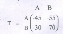
Where A represents the percentage of subscribers and B represents the percentage of non - subscribers.
A 40% = ·40
By the given data, 40% received the order of subscription = 60% are non-subscribers.
A 40% = ·40
and B 60% = ·60
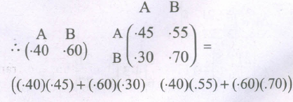
((-40)(-45) + (·60)(-30) (-40)(.55) + (-60)(.70))
(-18+·18 ·22+42)
(·36 ·64)
\(\Rightarrow\) 36% of those receiving the current letter can be expected to order a subscription
48.
Given non-homogeneous equations are
x + y + z = 3
x + 2y + 3z = 4
x + 4y + 9z = 6
The matrix equation corresponding to the given system is
\(\left( \begin{matrix} 1 & 1 & 1 \\ 1 & 2 & 3 \\ 11 & 4 & 9 \end{matrix} \right) \left( \begin{matrix} x \\ y \\ z \end{matrix} \right) =\left( \begin{matrix} 3 \\ 4 \\ 6 \end{matrix} \right) \)
AX = B
| Augmented matrix | Elementary Transformation |
|---|---|
| \(\left( \begin{matrix} 1 & 1 & 1 \\ 1 & 2 & 3 \\ 1 & 4 & 9 \end{matrix}\begin{matrix} 3 \\ 4 \\ 6 \end{matrix} \right) \) | |
| \(\left( \begin{matrix} 1 & 1 & 1 \\ 0 & 1 & 2 \\ 0 & 3 & 8 \end{matrix}\begin{matrix} 3 \\ 1 \\ R \end{matrix} \right) \) | \({ R }_{ 2 }\rightarrow { R }_{ 2 }-{ R }_{ 1 }\) \({ R }_{ 3 }\rightarrow { R }_{ 3 }-{ R_{ 1 } }\) |
| \(\left( \begin{matrix} 1 & 1 & 1 \\ 0 & 1 & 2 \\ 0 & 0 & 2 \end{matrix}\begin{matrix} 3 \\ 1 \\ 0 \end{matrix} \right) \) | \({ R }_{ 3 }\rightarrow { R }_{ 3 }-{ R }_{ 2 }\) |
Clearly the last equivalent matrix is in echelon form and it has three non-zero rows
\(\therefore \rho (A)=3\quad \rho \left( \left[ A,B \right] \right) =3\)
\(\rho (A)=\rho \left( \left[ A,B \right] \right) =3\)
\(\therefore\) The given system is consistent and has unique solution.
To find the solution, let us rewrite the above echelon form into the matrix form
\(\left( \begin{matrix} 1 & 1 & 1 \\ 0 & 1 & 2 \\ 0 & 0 & 2 \end{matrix} \right) \left( \begin{matrix} x \\ y \\ z \end{matrix} \right) =\left( \begin{matrix} 3 \\ 1 \\ 0 \end{matrix} \right) \)
\(\Rightarrow\) x + y + z = 3
y + 2z = 1
\((3)\Rightarrow 2x=0\Rightarrow z=\cfrac { 0 }{ 2 } =0\)
\((2)\Rightarrow y+2(0)=1\Rightarrow y+0=1\Rightarrow y=1-0=1\)
\(\left( 1 \right) \Rightarrow x+1+0=3\)
\(\Rightarrow x+1=3\)
\(\Rightarrow x=3-1\)
\(\Rightarrow x=2\)
\(\therefore\) Solution set [2, 1, 0]

12th Standard Syllabus & Materials
12th Standard
TN 12th Computer Applications களப்பெயர் முறைமை (DNS) Sample Question Papers Study Material - QB365 Set A
NEW12th Standard
TN 12th Computer Applications வலையமைப்பு எடுத்துக்காட்டுகள் மற்றும் நெறிமுறைகள் Sample Question Papers Study Material - QB365 Set A
NEW12th Standard
TN 12th Computer Applications கணினி வலையமைப்பு ஓர் அறிமுகம் Sample Question Papers Study Material - QB365 Set A
NEW12th Standard
TN 12th Computer Applications PHP-உடன் MySQL-ஐ இணைத்தல் Sample Question Papers Study Material - QB365 Set A



Tamilnadu Stateboard 12th Standard Subjects

Maths

Chemistry

Physics

Biology

Computer Science
Business Maths and Statistics

Economics

Commerce

Accountancy

History

Computer Applications
Biology
Computer Technology
Computer Applications
Computer Science
Business Maths and Statistics
Commerce
Economics
Maths
Chemistry
Physics
Computer Technology
History
Accountancy

Tamil

English

French
Tamilnadu Stateboard Standards
