
 100% FREE ACCESS
12th Standard Syllabus & Materials
12th Standard
TN 12th Computer Applications மின்னணு தரவு பரிமாற்றம் Sample Question Papers Study Material - QB365 Set A
NEW12th Standard
TN 12th Computer Applications மின் - வணிக பாதுகாப்பு அமைப்புகள் Sample Question Papers Study Material - QB365 Set A
NEW12th Standard
TN 12th Computer Applications மின்னணு செலுத்தல் முறைகள் Sample Question Papers Study Material - QB365 Set A
NEW12th Standard
TN 12th Computer Applications மின் - வணிகம் Sample Question Papers Study Material - QB365 Set A
NEW12th Standard
TN 12th Computer Applications திறந்த மூல கருத்துருக்கள் Sample Question Papers Study Material - QB365 Set A
NEW12th Standard
TN 12th Computer Applications வலையமைப்பு வடமிடல் Sample Question Papers Study Material - QB365 Set A

Published on: 01/03/2021
12th Standard English medium Business Maths Reduced Syllabus Two Mark Important Questions with Answer key - 2021(Public Exam )
Download Tamil Nadu 12th Standard Business Maths and Statistics question papers, model tests, one-mark questions, important questions, and public exam papers in PDF format. Free study materials and answer keys for TN State Board students.
Questions + Answers key
Take MCQ Business Maths and Statistics Test
1.
Find the order and degree of the following differential equation
\(\frac { { d }^{ 2 }y }{ { dx }^{ 2 } } -2\frac { dy }{ dx } +3y=0\)
2.
Evaluate the following
\(\int _{ 0 }^{ \infty }{ { e }^{ -mx } } { x }^{ 6 }dx\)
3.
What is the difference between Assignment Problem and Transportation Problem?
4.
5.
What is feasible solution and non degenerate solution in transportation problem?
6.
What are the uses of statistical quality control?
7.
Define R Chart.
8.
Name the control charts for variables.
9.
Define Family Budget Method.
10.
Define true value ratio.
11.
Define Time Reversal Test.
12.
State the test of adequacy of index number.
13.
Write note on Fisher’s price index number.
14.
Define Laspeyre’s price index number.
15.
Mention the classification of Index Number.
16.
Define seasonal index.
17.
Mention the components of the time series.
18.
State the uses of time series.
19.
Define Time series.
20.
Solve: (x2 + x + 1)dx + (y2− y + 3)dy = 0
21.
Define level of significance.
22.
Define critical value.
23.
What is confidence interval?
24.
What is point estimation?
25.
State any two demerits of systematic random sampling.
26.
What is standard error?
27.
Define parameter.
28.
What is sample?
29.
Define Standard normal variate.
30.
Write any 2 examples for Poisson distribution.
31.
A pair of dice is thrown 4 times. If getting a doublet is considered a success, find the probability of 2 successes.
32.
Write down the conditions for which the binomial distribution can be used.
33.
In tossing of a five fair coin, find the chance of getting exactly 3 heads.
34.
35.
Integrate the following with respect to x.
(4x + 2) \(\sqrt { { x }^{ 2 }+x+1 } \)
36.
How do you define variance in terms of Mathematical expectation?
37.
In an investment, a man can make a profit of Rs. 5,000 with a probability of 0.62 or a loss of Rs. 8,000 with a probability of 0.38. Find the expected gain.
38.
Explain the distribution function of a random variable.
39.
What do you understand by continuous random variable?
40.
Define random variable.
41.
The discrete random variable X has the probability function
| X | 1 | 2 | 3 | 4 |
| P(X=x) | k | 2k | 3k | 4k |
Show that k = 0.1.
42.
Suppose, the life in hours of a radio tube has the following p.d.f
\(f(x)=\left\{\begin{array}{l} \frac{100}{x^{2}}, \text { when } x \geq 100 \\ 0, \text { when } x<100 \end{array}\right.\)
Find the distribution function.
43.
Find the area bounded by the lines y − 2x − 4 = 0, y = 1, y = 3 and the y-axis
44.
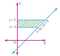
Find the area of the region bounded by the line x − 2y − 12 = 0 , the y-axis and the lines y = 2, y = 5.
45.
Integrate the following with respect to x.
(3 + x)(2 − 5x)
46.
Evaluate \(\int \sqrt{2 x+1} \ d x\)
47.
Find the rank of each of the following matrices.
\(\left( \begin{matrix} 5 & 6 \\ 7 & 8 \end{matrix} \right) \)
48.
For the marginal revenue function MR = 6 − 3x2 − x3, Find the revenue function and demand function.
49.
If MR = 14 − 6x + 9x2, find the demand function.
50.
A manufacturing company has found that the cost C of operating and maintaining the equipment is related to the length ‘m’ of intervals between overhauls by the equation m2\(\frac{dC}{dm}\) + 2mC = 2 and c = 4 and when m = 2. Find the relationship between C and m.
1.
\(\frac { { d }^{ 2 }y }{ { dx }^{ 2 } } -2\frac { dy }{ dx } +3y=0\)
Highest order derivative is \(\frac { { d }^{ 2 }y }{ d{ x }^{ 2 } }\)
∴ order = 2
Power of the highest order derivative \(\frac { { d }^{ 2 }y }{ d{ x }^{ 2 } }\) is 1
∴ Degree = 1
2.
Let I = \(\int _{ 0 }^{ \infty }{ { e }^{ -mx } } { x }^{ 6 }dx\)
Gamma Integral \(\int _{ 0 }^{ \infty }{ { x }^{ n } } { e }^{ -ax }dx=\frac { n! }{ { a }^{ n+1 } } \)
Here n = 6, and a = m
\(\therefore I=\int _{ 0 }^{ \infty }{ { e }^{ -mx } } { x }^{ 6 }dx\)
\(=\frac { 6! }{ { m }^{ 6+1 } } =\frac { 6! }{ { m }^{ 7 } } \)
3.
The assignment problem is a special case of transportation problem where the number of sources and destinations are equal. Here, jobs represent sources and machines represent destinations.
4.
5.
A feasible solution to a transportation problem is a set of non negative values xij (i = 1, 2, m, j = 1, 2, ....... n) that satisfies the constraints.
If a basic feasible solution to a transportation problem contains exactly m + n - l allocations. in independent positions, it is called a non degenerate basic feasible solution. Here m is the number of rows and n is the number of columns in a transportation problem.
6.
I. It is a powerful technique used to diagnose the lack of quality in any of the raw materials, process, machines etc.
II. It is essential that the end products should possess the qualities that the consumer expects from the manufacturer.
7.
The R chart is to show the variability or dispersion of the samples taken from the given process.
8.
The control charts of variables are
(i) Charts for mean (\(\overline { X } \))
(ii) Charts for Range (R)
9.
In this method, the weights are calculated by multiplying prices and quantity of the base year.
Cost of living index number = \(\frac {\sum pV}{\sum V}\) where
P = \(\frac {p_{1}}{p_{0}} \times 100 \) is the price relative and
V = \(\sum p_{0}q_{0}\) is the value relative
10.
The ratio between the total value of current period and total value of the base period is known as true value ratio.
(\( \frac{\sum P_{1} q_{1}}{\sum p_{0} q_{0}}\) is a true value tario)
11.
Time reversal test is an important test for testing the consistency of a good index number. This test maintains time consistency by working both forward and backward with respect to time (here time refers to base year and current year). Symbolically the following Relationship should be satisfied, P01 \(\times\) P10 = 1 Fisher's index number formula satisfies the above relationship
\(\text { i.e. } P_{01}=\frac{1}{P_{10}} \text { or } P_{01} \times P_{10}=1(\text { Except the factor } 100 \text { ) }\)
12.
Index numbers are studied to know the relative changes in price and quantity for any two years compared. There are two tests which are used to test the adequacy for an index number. The two tests are as follows.
(i) Time reversal test
(ii) Factor reversal test
The criterion for a good index number is to satisfy the above two tests.
13.
Fisher's price index number is the geometric mean of Laspeyre's and Paasche's price index number. Hence it is weighted index number.
Fisher's price index number = \(\sqrt {\frac {\sum p_{1}q_{0}}{\sum p_{0}q_{0} }}{\times}{\frac {\sum p_{1}q_{1}}{\sum p_{0}q_{1}} \times {100}}\)
14.
The weighted aggregate index number using base period weights is called Laspeyre’s price index number.
\(P_{01}^{L}=\frac{\sum p_{1} q_{0}}{\sum p_{0} q_{0}} \times 100\)
Where p1 is current year price
p0 is base year price
q0 is base year quantity
15.
Index number can be classified as follows
(i) Price index number
It measures the general changes in the retail or wholesale price level of a particular or group of commodities.
(ii) Quantity index number
These are indices to measure the changes in the quantity of goods manufactured in a factory.
(iii) Cost of living index number
These are intended to study the effect of change in the price level on the cost of living of diferent classes of people.
16.
Seasonal index is a measure of how a particular season compares with the average season.
17.
The components of time series are
(i) Secular trend
(ii) Seasonal variations
(iii) Cyclic variations
(iv) Irregular variations
18.
Time series has an important objective to identify the variations and try to eliminate the variations and also helps us to estimate or predict the future values.
19.
A time series consists of a set of observations arranged in chronological order (either ascending or descending). It is a statistical data which relates to successive intervals or point of time.
20.
Given (x2+ x + 1)dx + (y2−y + 3)dy = 0
It is of the form f(x)dx + g(y)dy = 0
Integrating , we get
ഽ(x2+ x + 1)dx + ഽ(y2 − y + 3)dy = c
\(\left( \frac { x^{ 3 } }{ 3 } +\frac { { x }^{ 2 } }{ 2 } +x \right) +\left( \frac { { y }^{ 3 } }{ 3 } -\frac { { y }^{ 2 } }{ 2 } +3y \right) =c\)
21.
The probability of type I error is known as level of significance denoted by \(\alpha\). It is always fixed in advance before collecting the sample information.
22.
The value of test statistic which separates the critical (or rejection) region and the acceptance region is called the critical value or significant value.
23.
The interval within which the unknown value of parameter is, expected to lie is called confidence interval. It indicates the probability that the population parameter lies within a specilied range. If o is the population paramcter, then we choose a small value a, known as level of significance (1% or 5%) and determine 2 constants c, and c,such that p(c1 < 0 < c2/t) = 1- \(\alpha\). When t is the value of statistic. The quantities c1 and c2 are determined as confidence limits and the interval [c1, c2] within which the unknown value of the population parameter is expected to lieis known as confidence interval.
24.
When a single value is used as an estimate, the estimate is called a point estimate of the population parameter In other words, an estimate of a population parameter given by a single numberis called as point estimation.
25.
1. Systematic samples are not random samples.
2. If N is not a multiple of n, then the sampling interval (k) cannot be an integer, thus sample selection becomes difficult.
26.
The standard deviation of the sampling distribution of a statistic is known as its Standard Error.
27.
The statistical constants of the population like mean (μ), variance (σ2) are referred as population parameters.
28.
A selection of a group of individuals from a population in such a way that it represents the population is called as sample.
29.
A random variable Z = \(\frac { X-\mu }{ \sigma } \) follows the standard normal distribution is called the standard normal variate with mean 0 and standard deviation 1. i.e. Z~ N(0,1). Its,probability density function is given by:
\(\varphi(Z)=\frac{1}{\sqrt{2 \pi}} e^{-\frac{Z^{2}}{2}},-\infty< Z< \infty
\)
30.
(i) Number of lightnings per second.
(ii) Number of printing mistakes per page in a textbook.
31.
Let p be the probability of getting doublet in a pair of dice.
∴ p = \(\frac { 6 }{ 36 } \) [∵ favourable events are (1, 1) (2,2) (3,3) (4,4) (5,5) (6,6) and n(S) = 36]
⇒ p = \(\frac { 1 }{ 6 } \) ∴ q=1-p =\(1-\frac { 1 }{ 6 } =\frac { 5 }{ 6 } \)]
∴ P (getting 2 success) = P(X = 2)
=4C2 \(\left( \frac { 1 }{ 6 } \right) ^{ 2 }\left( \frac { 5 }{ 6 } \right) ^{ 2 }\) [∵ p(x) =nCx pxqn-x, n = 4, x = 2 ]
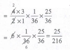
∴ P(X = 2) =\(\frac { 25 }{ 216 } \).
32.
The binomial distribution can be used under the following conditions.
(i) The number of trials en' is finite,
(ii) The trials are independent of each other.
(iii) The probability of success 'p' is constant for each trial.
(iv) In every trial there are only two possible outcomes namely success or failure.
33.
Let X be a random variable follows binomial distribution with p = q = 1/2
P (3 heads) = \(5{ C }_{ x }{ \left( \frac { 1 }{ 2 } \right) }^{ x }{ \left( \frac { 1 }{ 2 } \right) }^{ 5-x }\)
\(={ 5C }_{ 3 }{ \left( \frac { 1 }{ 2 } \right) }^{ 3 }{ \left( \frac { 1 }{ 2 } \right) }^{ 5-3 }\)
\(=5{ C }_{ 3 }{ \left( \frac { 1 }{ 2 } \right) }^{ 5 }\)
\(=\frac { 5 }{ 16 } \)
34.
35.
\(Let\ I=\int { \left( 4x+2 \right) } \sqrt { { x }^{ 2 }+x+1 } \ dx\)
\(put\ t={ x }^{ 2 }+x+1\)
dt = (2x+1) dx
\(\therefore I=2\int { \left( 2x+1 \right) } \sqrt { { x }^{ 2 }+x+1 } \ dx\)
\(=2\int { \sqrt { t } } dt\)
\(=2\int { { t }^{ \frac { 1 }{ 2 } } } dt=2\frac { { t }^{ \frac { 1 }{ 2 } +1 } }{ \frac { 1 }{ 2 } +1 } +c\)
\(=2\frac { { t }^{ \frac { 3 }{ 2 } } }{ \frac { 3 }{ 2 } } +c\)
\(=\frac { 4 }{ 3 } { t }^{ \frac { 3 }{ 2 } }+c\)
\(=\frac { 4 }{ 3 } { \left( { x }^{ 2 }+x+1 \right) }^{ \frac { 3 }{ 2 } }+c\quad \left[ \because t={ x }^{ 2 }+x+1 \right] \)
36.
Var (X) = E(X2) - [E(X)]2 where
\(E({ X }^{ 2 })=\begin{cases} \sum { { x }^{ 2 }p(x)\text {for discrete random variable} } \\ \int _{ -\infty }^{ \infty }{ { x }^{ 2 }P(x)\text{dx for continuous random variable} } \end{cases}\)
37.
Given that in an investment profit is Rs. 5000 with probability of 0.62 or a loss of Rs.8000 with a probability of 0.38.
Hence, the probability mass function is
| X = x | 5000 | -8000 |
| P(X = x) | 0.61 | 0.38 |
∴ Expected gain E(X) = 5000(0.62) - 8000 (0.32)
= 3100-3040
= Rs. 60
Hence, the expected gain is = Rs. 60
38.
The discrete cumulative distribution function or distribution function of a real valued discrete random variable X takes the countable number of points x1,x2, .... with corresponding probabilities p(x1)p(x2).... and the distribution function is defined by
Fx(x) = P(X≤x) for all x∈R
ie.Fx(x) = \(\sum _{ { x }_{ i }\le x }^{ }{ p({ x }_{ i }) } \)
For a continuous random variable with the probability density function fx(x) then the distribution function Fx(x) is defined by
Fx(x) = P(X≤x)
39.
Continuous random variable :
A random variable X which can take on any value (integral as well as fraction) in the interval is called continuous random variable. For eg., height of students in a school.
40.
A random variable is a real valued function defined on a sample space S and taking values in (-∞, ∞) or whose possible values are numerical outcomes of a random experiment.
41.
The given probability function is
| X | 1 | 2 | 3 | 4 |
| P(X = x) | k | 2k | 3k | 4k |
Since the given function is a probability function, each ρi>0 and Σρi = 1
⇒ k + 2k + 3k + 4k = 1
⇒10k = 1 ⇒ k = \(\frac{1}{10}\)
⇒ k = 0.1
42.
\(F(x)=\int _{ -\infty }^{ x }{ f(t)dt } \)
\(=\int _{ 100 }^{ x }{ \frac { 100 }{ { t }^{ 2 } } dt,\quad x\ge 100 } \)
\(={ \left[ \frac { 100 }{ -t } \right] }_{ 100 }^{ x },\quad x\ge 100\)
\(F(x)=\left[ 1-\frac { 100 }{ x } \right] ,\ge 100\)
43.
y - 2x - 4 = 0
| x | 0 | -2 |
| y | 4 | 0 |
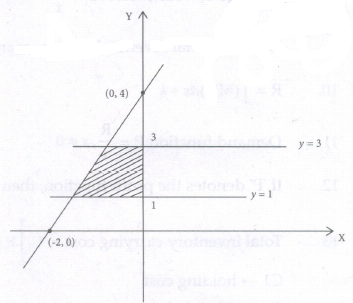
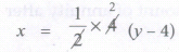
Given y - 2.x - 4 = 0
⇒ y-4 = 2x
⇒
Since the area lies to the left of Y-axis, with the limits y = 1 &y = 3.
Area =\(\int _{ 1 }^{ 3 }{ -xdy } \)
\(=\int _{ 1 }^{ 3 }{ -\left( \frac { 1 }{ 2 } \right) (y-4)dy } \)
\(=\frac { 1 }{ 2 } \int _{ 1 }^{ 3 }{ (4-y)dy } =\frac { 1 }{ 2 } { \left[ 4y-\frac { { y }^{ 2 } }{ 2 } \right] }_{ 1 }^{ 3 }\)
\(=\frac { 1 }{ 2 } \left[ \left( 4(3)-\frac { { 3 }^{ 2 } }{ 2 } \right) -\left( 4(1)-\frac { { 1 }^{ 2 } }{ 2 } \right) \right] \)
\(=\frac { 1 }{ 2 } \left[ \left( 12-\frac { 9 }{ 2 } \right) -\left( 4-\frac { 1 }{ 2 } \right) \right] \)
\(=\frac { 1 }{ 2 } \left[ \left( \frac { 24-9 }{ 2 } \right) -\left( \frac { 8-1 }{ 2 } \right) \right] \)
\(=\frac { 1 }{ 2 } \left[ \frac { 15 }{ 2 } -\frac { 7 }{ 2 } \right] =\frac { 1 }{ 2 } \left[ \frac { 8 }{ 2 } \right] \)
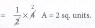
44.
x - 2y - 12 = 0
x = 2y + 12
Required Area
= \(\int _{ 2 }^{ 5 }{ xdy } \)
= \(\int _{ 2 }^{ 5 }{ (2y+12)dy= } [{ { y }^{ 2 }+12y] }_{ 2 }^{ 5 }\)
= (25 + 60)−(4 + 24) = 57 sq.units
45.
\(\int { \left( 3x+x \right) \left( 2-5x \right) } dx\)
\(=\int { \left( 6-15x+2x-{ 5x }^{ 2 } \right) } dx\)
\(=\int { \left( 6-13x-{ 5x }^{ 2 } \right) } dx\)
\(=6x-\frac { { 13x }^{ 2 } }{ 2 } -\frac { { 5x }^{ 3 } }{ 3 } +c\)
46.
\( \int \sqrt{2 x+1} \ d x=\int(2 x+1)^{\frac{1}{2}} d x\)
\(=\frac { { \left( 2x+1 \right) }^{ \frac { 3 }{ 2 } } }{ 3 } +c\)
47.
Let \(A=\left( \begin{matrix} 5 & 6 \\ 7 & 8 \end{matrix} \right) \)
Order of A is 2 \(\times\) 2
\(\therefore \rho (A)\le 2\) [Since minimum of (2, 2) is 2]
Consider the second order minor
\(\left| \begin{matrix} 5 & 6 \\ 7 & 8 \end{matrix} \right| =40-42\)
= \(-2\neq 0\)
There is a minor of order 2, which is not zero
\(\therefore \rho (A)=2\)
48.
Given MR = 6 − 3x2 − x3
⇒ ഽMR =ഽ(6 − 3x2 − x3)dx
\(\Rightarrow \mathrm{R}=6 x-\frac{\not{3} x^{3}}{\not3}-\frac{x^{4}}{4}+k\)
\(\Rightarrow 6x-{ x }^{ 3 }-\frac { { x }^{ 4 } }{ 4 } +k\)
When x = 0, R = 0 ⇒ k = 0
\(\Rightarrow R=6x-{ x }^{ 3 }-\frac { { x }^{ 4 } }{ 4 } \)
Demand function \(P=\frac { R }{ x } =6-{ x }^{ 2 }-\frac { { x }^{ 3 } }{ 4 } \)
49.
Given MR = 14 - x + 9x2
⇒ \(\frac{dR}{dx}\) = 14 - 6x + 9x2
⇒ dR = (14 - 6x + 9x2)dx
⇒ ഽdR = ഽ(14 - 6x + 9x2)dx
\(\Rightarrow \ R=14x-\frac { 6{ x }^{ 2 } }{ 2 } +\frac { { 9x }^{ 3 } }{ 3 } +k\)
When x = 0, R = 0 ⇒ k = 0
R = 14x - 3x2+ 3x3
Demand function \(P=\frac { R }{ x } =\frac { 14x-3{ x }^{ 2 }+{ 3x }^{ 3 } }{ x } \)
⇒ P = 14 − 3x + 3x2
50.
Given m2\(\frac { dc }{ dm } \)+2mc = 2
Dividing by m2, we get,
\(\frac { dC }{ dm } +\frac { 2c }{ m } =\frac { 2 }{ { m }^{ 2 } } \)
This is of form \(\frac { dy }{ dx } \)+Py = Q
where P = \(\frac { 2 }{ m } \) and Q = \(\frac { 2 }{ m } \)
\(\int { p } dm=\int { \frac { 2 }{ m } } \)dm = 2 log m = log m2
∴ Integrating Factor (LF.) = \(e^{ \int { P } dm }=e^{ logm^{ 2 } }\)
= m2
∴ The solution is
\(ce^{ \int { P } dm }=\int { Q } e^{ \int { P } dm }m+c.K\)
cm2=\(\int { \frac { 2 }{ { m }^{ 2 } } { m }^{ 2 } } dm+K=\int { 2 } dm+cK\)
cm2 = 2m+K
Given that c = 4, when m = 2
4(22) = 2(2) + K ⇒ 16 - 4 = K
⇒ K=12
∴ (1) becomes
cm2 = 2m+ 12
⇒ cm2 = 2 (m + 6)

12th Standard Syllabus & Materials
12th Standard
TN 12th Computer Applications களப்பெயர் முறைமை (DNS) Sample Question Papers Study Material - QB365 Set A
NEW12th Standard
TN 12th Computer Applications வலையமைப்பு எடுத்துக்காட்டுகள் மற்றும் நெறிமுறைகள் Sample Question Papers Study Material - QB365 Set A
NEW12th Standard
TN 12th Computer Applications கணினி வலையமைப்பு ஓர் அறிமுகம் Sample Question Papers Study Material - QB365 Set A
NEW12th Standard
TN 12th Computer Applications PHP-உடன் MySQL-ஐ இணைத்தல் Sample Question Papers Study Material - QB365 Set A



Tamilnadu Stateboard 12th Standard Subjects

Maths

Chemistry

Physics

Biology

Computer Science
Business Maths and Statistics

Economics

Commerce

Accountancy

History

Computer Applications
Biology
Computer Technology
Computer Applications
Computer Science
Business Maths and Statistics
Commerce
Economics
Maths
Chemistry
Physics
Computer Technology
History
Accountancy

Tamil

English

French
Tamilnadu Stateboard Standards
