
 100% FREE ACCESS
12th Standard Syllabus & Materials
12th Standard
TN 12th Computer Applications மின்னணு தரவு பரிமாற்றம் Sample Question Papers Study Material - QB365 Set A
NEW12th Standard
TN 12th Computer Applications மின் - வணிக பாதுகாப்பு அமைப்புகள் Sample Question Papers Study Material - QB365 Set A
NEW12th Standard
TN 12th Computer Applications மின்னணு செலுத்தல் முறைகள் Sample Question Papers Study Material - QB365 Set A
NEW12th Standard
TN 12th Computer Applications மின் - வணிகம் Sample Question Papers Study Material - QB365 Set A
NEW12th Standard
TN 12th Computer Applications திறந்த மூல கருத்துருக்கள் Sample Question Papers Study Material - QB365 Set A
NEW12th Standard
TN 12th Computer Applications வலையமைப்பு வடமிடல் Sample Question Papers Study Material - QB365 Set A

Published on: 13/05/2022
QB365 provides detailed and simple solution for every book back questions in class 12 Maths subject.It will helps to get more idea about question pattern in every book back questions with solution.
latest Book back QuestionsDownload Tamil Nadu 12th Standard Maths question papers, model tests, one-mark questions, important questions, and public exam papers in PDF format. Free study materials and answer keys for TN State Board students.
Questions + Answers key
Take MCQ Maths Test1.
A steel plant is capable of producing x tonnes per day of a low-grade steel and y tonnes per day of a high-grade steel, where \(y=\frac { 40-5x }{ 10-x } \). If the fixed market price of low-grade steel is half that of high-grade steel, then what should be optimal productions in low-grade steel and high-grade steel in order to have maximum receipts.
2.
Evaluate the following limit, if necessary use l ’Hôpital Rule
\(\underset { x\rightarrow { \frac { \pi }{ 2 } } }{ lim } { \left( sinx \right) }^{ tanx }\)
3.
Write the Maclaurin series expansion of the following function
tan-1(x); -1 ≤ x ≤ 1
4.
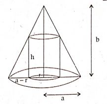
5.
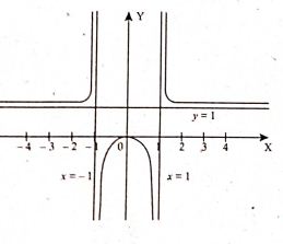
Find the asymptotes of the following curve \(f(x)=\frac { { x }^{ 2 } }{ { x }^{ 2 }-1 } \)
1.
Let the price of low-grade steel be Rs. p per tonne. Then the price of high-grade steel is Rs. 2p per tonne.
The total receipt per day is given by \(R=px+py=px+2p\left( \frac { 40-5x }{ 10-x } \right) \). Hence the problem is to maximise R . Now, simplifying and differentiating R with respect to x , we get
\(R=p\left( \frac { 80-{ x }^{ 2 } }{ 10-x } \right) \)
\(\frac { dR }{ dx } =p\left( \frac { { x }^{ 2 }-20x+80 }{ (10-x)^{ 2 } } \right) \)
\(\frac { dR }{ dx } =-\frac { 40P }{ \left( 10-x \right) ^{ 3 } } \)
Now, \(\frac { dR }{ dx } =0\Rightarrow { x }^{ 2 }-20x+80=0\) and hence \(x=10\pm 2\sqrt { 5 } \)
At \(x=10-2\sqrt { 5 } ,\frac { { d }^{ 2 }R }{ { dx }^{ 2 } } <0\) and hence R will be maximum. If x \(x=10-2\sqrt { 5 } \) then \(y=5-\sqrt { 5 } \)
Therefore the steel plant must produce low-grade and high-grade steels respectively in tonnes per day are \(10-2\sqrt { 5 } \) and \(5-5\sqrt { 5 } \)
2.
This is an indeterminate of the from 1∞
Let g(x) = (sin x)tan x
Taking logarithm, we get
log (g(x)) = log (sin x)tan x
= tan x log (sin x)
Now, \(\underset { x\rightarrow { \frac { \pi }{ 2 } } }{ lim } log(g(x))\) = \(\underset { x\rightarrow { \frac { \pi }{ 2 } } }{ lim } \frac { log(sinx) }{ cotx } =\left( \frac { 0 }{ 0 } form \right) \)
= \(\frac { \underset { x\rightarrow { \frac { \pi }{ 2 } } }{ lim } \frac { 1 }{ sinx } \times cosx }{ -{ cosec }^{ 2 }x } \) [By L' Hôpital Rule]
= \(\underset { x\rightarrow { \frac { \pi }{ 2 } } }{ lim } -\frac { cosx }{ sinx\frac { 1 }{ { sin }^{ 2 }x } } \)
= \(\underset { x\rightarrow { \frac { \pi }{ 2 } } }{ lim } cos \ x \ sin \ x=0\)
But \(\underset { x\rightarrow { \frac { \pi }{ 2 } } }{ lim } log(g(x))=log(\underset { x\rightarrow { \frac { \pi }{ 2 } } }{ lim } g(x))\)
\(\therefore log\left( \underset { x\rightarrow { \frac { \pi }{ 2 } } }{ lim } g(x) \right) =log \ 0=1\)
\(\Rightarrow { e }^{ log }\left( \underset { x\rightarrow { \frac { \pi }{ 2 } } }{ lim } g(x) \right) ={ e }^{ 1 }\)
\(\Rightarrow \underset { x\rightarrow { \frac { \pi }{ 2 } } }{ lim } g(x)=e\Rightarrow \underset { x\rightarrow { \frac { \pi }{ 2 } } }{ lim } { (sinx) }^{ tanx }=e^o=1\)
3.
Let f(x) = tan-1(x)
⇒ f(0) = tan-1(0) = 0
\({ f }^{ -1 }(x)=\frac { 1 }{ 1+{ x }^{ 2 } } ={ (1+{ x }^{ 2 }) }^{ -1 }\)
⇒ fI(0) = 1
fII(x) = -1(1 + x)-2 (2x)
= -2x(1 + x2)-2
⇒ fII(0) = 0
= -2[-4x2(1 + x2)-3 + (1 + x2)-2]
fIII(x) = -2[x(-2)(1+x2)-3 (2x) + (1 + x2)-2]
⇒ fIII(0) = 2
fIV(x) = -2[-4x2(-3) (1 + x2)-4 (2x) + (1 + x2)-3(-8x) + (1 + x2)-3(-2)(2x)]
⇒ fIIl(0) = 2
= - 2 [24x3 (1 + x2)-4-8x (1+ x2)3 -4x (1 + x2)3]
= - 2 [24x3 (1 + x2)-4-12x (1+ x2)3]
fIV(x) = 24[2x3 (1 + x2)-4 - x (1 + x2)-3]
⇒ fIl(0) = 0
fV(x) = - 24 [2x3 (-4)(1 +x2)-5(2x) + (1+ x2)-4(6x2 -x (- 3)(1 + x2)-4(2x) - (1 + x2)3]
= - 24 [16x4 (1 + x2)-5+ 6x2 (1+ x2)-4- (1 + x2)3]
= - 24 [16x4 (1 + x2)-5+12x2 (1+ x2)-4- (1 + x2)3]
⇒ fV(0) = 24
⇒ f(0) = tan-1 (0) = 0
⇒ fI(0) = 1
⇒ fII(0) = 0
⇒ fIII(0) = -2
⇒ fIV(0) = 0
⇒ fV(0) = 24
Maclaurin's series
\(f(x)=f(0)+\frac { { f }^{ 1 }(0) }{ 1! } x+\frac { { f }^{ II }(0) }{ 2! } { x }^{ 2 }+\frac { { f }^{ III }(0) }{ 3! } { x }^{ 3 }+\frac { { f }^{ IV }(0) }{ 4! } { x }^{ 4 }+..\)
= \(0+\frac { 1 }{ 1! } x+0\frac { 2 }{ 3! } { x }^{ 3 }+0+\frac { 24 }{ 5! } { x }^{ 5 }+\)...
= x - \(\frac { { x }^{ 3 } }{ 3 } +\frac { { x }^{ 5 } }{ 5 } +\).......
4.
5.
Given \(f(x)=\frac { { x }^{ 2 } }{ { x }^{ 2 }-1 } \)
\(\quad \underset { x\rightarrow 1^{ + } }{ lim } \frac { { x }^{ 2 } }{ { x }^{ 2 }-1 } =\underset { x\rightarrow 1^{ + } }{ lim } \frac { { x }^{ 2 } }{ \left( x+1 \right) \left( x-1 \right) } \)
= \(\underset { h\rightarrow { 0 }^{ + } }{ lim } \frac { \left( 1+h \right) ^{ 2 } }{ \left( 1+h+1 \right) \left( 1+h-1 \right) } \)
= \(\underset { h\rightarrow 0^{ + } }{ lim } \frac { (1+h)^{ 2 } }{ (2+h)(h) } \infty \)
Also \(\underset { x\rightarrow 1^{ - } }{ lim } \frac { { x }^{ 2 } }{ (x+1)/(x-1) } =\underset { h\rightarrow 0^{ + } }{ lim } \frac { \left( 1-h \right) ^{ 2 } }{ \left( 1-h+1 \right) \left( 1-h-1 \right) } \)
= \(\underset { h\rightarrow { 0 }^{ + } }{ lim } \frac { \left( 1-h \right) ^{ 2 } }{ (2-h)(-h) } =-\infty \)
ஃ x = -1 and x = 1are vertical asymptotes,
Also
\(\underset { x-\rightarrow \infty }{ lim } \frac { { x }^{ 2 } }{ { x }^{ 2 }-1 } =\underset { \frac { 1 }{ x } \rightarrow 0 }{ lim } \frac { 1 }{ 1-\frac { 1 }{ { x }^{ 2 } } } =1\)
[Divide numerator and denominator by x2]
ஃ y = 1 is a horizontal asymptote,

12th Standard Syllabus & Materials
12th Standard
TN 12th Computer Applications களப்பெயர் முறைமை (DNS) Sample Question Papers Study Material - QB365 Set A
NEW12th Standard
TN 12th Computer Applications வலையமைப்பு எடுத்துக்காட்டுகள் மற்றும் நெறிமுறைகள் Sample Question Papers Study Material - QB365 Set A
NEW12th Standard
TN 12th Computer Applications கணினி வலையமைப்பு ஓர் அறிமுகம் Sample Question Papers Study Material - QB365 Set A
NEW12th Standard
TN 12th Computer Applications PHP-உடன் MySQL-ஐ இணைத்தல் Sample Question Papers Study Material - QB365 Set A



Tamilnadu Stateboard 12th Standard Subjects
Maths

Chemistry

Physics

Biology

Computer Science

Business Maths and Statistics

Economics

Commerce

Accountancy

History

Computer Applications
Biology
Computer Technology
Computer Applications
Computer Science
Business Maths and Statistics
Commerce
Economics
Maths
Chemistry
Physics
Computer Technology
History
Accountancy

Tamil

English

French
Tamilnadu Stateboard Standards



