
 100% FREE ACCESS
12th Standard Syllabus & Materials
12th Standard
TN 12th Maths Applications of Matrices and Determinants Sample Question Papers Study Material - QB365 Set A
NEW12th Standard
TN 12th Computer Applications மின்னணு தரவு பரிமாற்றம் Sample Question Papers Study Material - QB365 Set A
NEW12th Standard
TN 12th Computer Applications மின் - வணிக பாதுகாப்பு அமைப்புகள் Sample Question Papers Study Material - QB365 Set A
NEW12th Standard
TN 12th Computer Applications மின்னணு செலுத்தல் முறைகள் Sample Question Papers Study Material - QB365 Set A
NEW12th Standard
TN 12th Computer Applications மின் - வணிகம் Sample Question Papers Study Material - QB365 Set A
NEW12th Standard
TN 12th Computer Applications திறந்த மூல கருத்துருக்கள் Sample Question Papers Study Material - QB365 Set A

Published on: 02/02/2021
12th Standard Maths English Medium Probability Distributions Reduced Syllabus Important Questions With Answer Key 2021
Download Tamil Nadu 12th Standard Maths question papers, model tests, one-mark questions, important questions, and public exam papers in PDF format. Free study materials and answer keys for TN State Board students.
Questions + Answers key
Take MCQ Maths Test1.
Find the binomial distribution function for each of the following.
(i) Five fair coins are tossed once and X denotes the number of heads.
(ii) A fair die is rolled 10 times and X denotes the number of times 4 appeared.
2.
If X is the random variable with distribution function F(x) given by,
\(F(x)=\begin{cases} \begin{matrix} 0 & x<0 \end{matrix} \\ \begin{matrix} x & 0\le x<1 \end{matrix} \\ \begin{matrix} 1 & 1\le x \end{matrix} \end{cases}\)
then find
(i) the probability density function f(x)
(ii) P(0.2 ≤ X ≤ 0.7)
3.
Two fair coins are tossed simultaneously (equivalent to a fair coin is tossed twice). Find the probability mass function for number of heads occurred.
4.
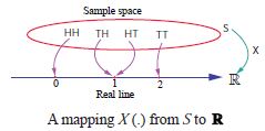
Suppose two coins are tossed once. If X denotes the number of tails,
(i) write down the sample space
(ii) find the inverse image of 1
(iii) the values of the random variable and number of elements in its inverse images
5.
6.
A six sided die is marked '2' on one face, '3' on two ofits faces, and '4' on remaining three faces. The die is thrown twice. If X denotes the total score in two throws, find the values of the random variable and number of points in its inverse images.
7.
In a pack of 52 playing cards, two cards are drawn at random simultaneously. If the number of black cards drawn is a random variable, find the values of the random variable and number of points in its inverse images.
8.
Find the mean and variance of a random variable X , whose probability density function is \(f(x)=\begin{cases} \begin{matrix} { \lambda e }^{ -2x } & for\ge 0 \end{matrix} \\ \begin{matrix} 0 & otherwise \end{matrix} \end{cases}\)
9.
The probability density function of random variable X is given by \(f(x)=\begin{cases} \begin{matrix} k & 1\le x\le 5 \end{matrix} \\ \begin{matrix} 0 & otherwise \end{matrix} \end{cases}\) Find
(i) Distribution function
(ii) P(X < 3)
(iii) P(2 < X < 4)
(iv) P(3 ≤ X )
10.
A random variable X has the following probability mass function
| x | 1 | 2 | 3 | 4 | 5 | 6 |
| f(x) | k | 2k | 6k | 5k | 6k | 10k |
Find
(i) P(2 < X < 6)
(ii) P(2 ≤ X < 5)
(iii) P(X ≤4)
(iv) P(3 < X )
11.
If the probability mass function f(x) of a random variable X is
| x | 1 | 2 | 3 | 4 |
| f (x) | \(\cfrac { 1 }{ 12 } \) | \(\cfrac { 5 }{ 12 } \) | \(\cfrac { 5 }{ 12 } \) | \(\cfrac { 1 }{ 12 } \) |
find (i) its cumulative distribution function, hence find
(ii) P(X ≤ 3) and,
(iii) P(X ≥ 2)
12.
If the probability that a fluorescent light has a useful life of at least 600 hours is 0.9, find the probabilities that among 12 such lights
(i) exactly 10 will have a useful life of at least 600 hours
(ii) at least 11 will have a useful life of at least 600 hours
(iii) at least 2 will not have a useful life of at least 600 hours.
13.
If the probability that a fluorescent light has a useful life of at least 600 hours is 0.9, find the probabilities that among 12 such lights
(i) exactly 10 will have a useful life of at least 600 hours;
(ii) at least 11 will have a useful life of at I least 600 hours;
(iii) at least 2 will not have a useful life of at : least 600 hours.
14.
The probability density function of X is given
\(f(x)=\begin{cases} \begin{matrix} { Ke }^{ \frac { -x }{ 3 } } & \begin{matrix} for & x>0 \end{matrix} \end{matrix} \\ \begin{matrix} 0 & \begin{matrix} for & x\le 0 \end{matrix} \end{matrix} \end{cases}\)
Find
(i) the value of k
(ii) the distribution function.
(iii) P(X <3)
(iv) P(5 ≤X)
(v) P(X ≤ 4)
15.
The probability that a certain kind of component will survive a electrical test is \(\frac { 3 }{ 4 } \). Find the probability that exactly 3 of the 5 components tested survive.
16.
Compute P(X = k) for the binomial distribution, B(n, p) where
n = 9, \(p=\frac { 1 }{ 2 } \), k = 7
17.
For the random variable X with the given probability mass function as below, find the mean and variance
\(f(x)= \begin{cases}2(x-1) & 1<x<2 \\ 0 & \text { otherwise }\end{cases}\)\(\)
18.
19.
A die is thrown 10 times. Getting a number greater than 3 is considered a success. The S.D of the number of successes is _________
2.5
1.56
5
25
20.
If the mean and variance of a binomial variate are 2 and 1 respectively, the probability that X takes a value greater than one is equal to__________.
\(\frac { 5 }{ 16 } \)
\(\frac { 11 }{ 16 } \)
\(\frac { 10 }{ 16 } \)
\(\frac { 1 }{ 2 } \)
21.
Var (2x ± 5) is =________
5
var (2x) ± 5
4 var (X)
0
22.
A die is tossed 5 times. Getting an odd number is considered a success. Then the variance of distribution of number of success is _____________
\(\frac { 8 }{ 3 } \)
\(\frac { 3 }{ 8 } \)
\(\frac { 4 }{ 5 } \)
\(\frac { 5 }{ 4 } \)
23.
In a binomial distribution, if the mean is 8 and the variance is 6, then the number of trials is _____________
32
48
16
12
24.
If \(f(x)=\frac { 1 }{ 2 } \) ,\(E\left( { x }^{ 2 } \right) =\frac { 1 }{ 4 } \) then var(x) is _____________
0
\(\frac { 1 }{ 4 } \)
\(\frac { 1 }{ 2 } \)
1
25.
26.
Let X have a Bernoulli distribution with mean 0.4, then the variance of (2X - 3) is
0.24
0.48
0.6
0.96
27.
28.
The random variable X has the probability density function
\(f(x)=\left\{\begin{array}{lr}
a x+b & 0<x<1 \\
0 & \text { otherwise }
\end{array}\right.\) and \(E(X)=\frac { 7 }{ 12 } \), then a and b are respectively
1 and \(\frac { 1 }{ 2 } \)
\(\frac { 1 }{ 2 } \) and 1
2 and 1
1 and 2
29.
If X is a binomial random variable with expected value 6 and variance 2.4, then P(X = 5) is
\(\left( \frac { 10 }{ 5 } \right) \left( \frac { 3 }{ 5 } \right) ^{ 6 }\left( \frac { 2 }{ 5 } \right) ^{ 4 }\)
\(\left( \frac { 10 }{ 5 } \right) \left( \frac { 3 }{ 5 } \right) ^{ 10 }\)
\(\left( \frac { 10 }{ 5 } \right) { \left( \frac { 3 }{ 5 } \right) }^{ 4 }\left( \frac { 2 }{ 5 } \right) ^{ 6 }\)
\(\left( \frac { 10 }{ 5 } \right) \left( \frac { 3 }{ 5 } \right) ^{ 5 }\left( \frac { 2 }{ 5 } \right) ^{ 5 }\)
30.
31.
32.
A random variable X has binomial distribution with n = 25 and p = 0.8 then standard deviation of X is
6
4
3
2
1.
(i) Given that five fair coins are tossed once. Since the coins are fair coins the probability of getting an head in a single coin is
\(p=\frac { 1 }{ 2 } \) and \(q=1-p=\frac { 1 }{ 2 } \)
Let X denote the number of heads that appear in five coins. X is binomial random variable that takes on the values 0, 1, 2, 3, 4 and 5 and \(p=\frac { 1 }{ 2 } \) That is \(X\sim B\left( 5,\cfrac { 1 }{ 2 } \right) \)
Therefore the binomial distribution is
\(f(x)=\left( \begin{matrix} n \\ x \end{matrix} \right) p*\left( 1-p \right) ^{ n-x }\), x = 0, 1, 2,..,n
becomes
\(f(x)=\left( \begin{matrix} 5 \\ x \end{matrix} \right) \left( \cfrac { 1 }{ 2 } \right) ^{ x }\left( \cfrac { 1 }{ 2 } \right) ^{ n-x }\), x = 0, 1, 2,..,5
That is
\(f(x)=\left( \begin{matrix} 5 \\ x \end{matrix} \right) \left( \cfrac { 1 }{ 2 } \right) ^{ n }\), x = 0, 1, 2...,n
(ii) A fair die is rolled ten times and X denotes the number of times 4 appeared. X is binomial
random variable that takes on the values 0, 1, 2, 3,...10 , with n = 10 and \(p=\cfrac { 1 }{ 6 } \). That is \(X\sim B\left( 10,\cfrac { 1 }{ 6 } \right) \)
Probability of getting a four in a die is \(p=\frac { 1 }{ 2 } \) and \(q=1-p=\frac { 5 }{ 6 } \)
Therefore the binomial distribution is
\(f(x)=\left( \begin{matrix} 10 \\ x \end{matrix} \right) \left( \cfrac { 1 }{ 6 } \right) ^{ x }\left( \cfrac { 5 }{ 6 } \right) ^{ 10-x }\) x = 0, 1, 2,...,10
2.
(i) Differentiating F(x) with respect to x at continuity points of f(x), we get
\(f(x)={ F }^{ 1 }(x)=\begin{cases} \begin{matrix} 0 & x<0 \end{matrix} \\ \begin{matrix} 1 & 0\le x<1 \end{matrix} \\ \begin{matrix} 0 & x\ge 1 \end{matrix} \end{cases}\)
The pdf f(x) is not continuous at x = 0, or at x = 1. We can define f(0) and f(1) in any manner. Choosing f(0) = 1, and f(1) = 0 .
Therefore the probability density function f(x) is
\(f(x)=\begin{cases} \begin{matrix} 1 & 0\le x<1 \end{matrix} \\ \begin{matrix} 0 & otherwise \end{matrix} \end{cases}\)
(ii) P(0.2 ≤ X ≤ 0.7) = F(0.7) − F(0.2)
= 0.7-0.2 = 0.5
\(P(0.2\le X\le 0.7)=\int _{ 0.2 }^{ 0.7 }{ f(x) } dx=\int _{ 0.2 }^{ 0.7 }{ 1dx } =0.5\)
3.
The sample space S = {H,T} \(\times\) {H,T}
That is S = {TT, TH, HT, HH}
Let X be the random variable denoting the number of heads.
Therefore
X (TT ) = 0 , X (TH ) = 1,
X (HT) = 1, and X (HH) = 2 .
Then the random variable X takes on the values 0, 1 and 2
| Values of the Random Variable | 0 | 1 | 2 | Total |
| Number of elements in inverse images | 1 | 2 | 1 | 4 |
The probabilities are given by
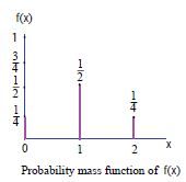
\(f(0)=P(X=0)=\cfrac { 1 }{ 4 } \)
\(f(1)=P(X=1)=\cfrac { 1 }{ 2 } \)
and \(f(2)=P(X=2)=\cfrac { 1 }{ 4 } \)
The function f (x) satisfies the conditions
(i) f (x) ≥ 0 , for x = 0, 1, 2
(ii) \(\underset { x }{ \Sigma } f(x)=\sum _{ x=0 }^{ x=2 }{ f(x) } =f(0)+f(1)+f(2)\)
= \(\cfrac { 1 }{ 4 } +{ \cfrac { 1 }{ 2 } +\cfrac { 1 }{ 4 } =1 }\)
Therefore f (x) is a probability mass function.
The probability mass function is given by
| x | 0 | 1 | 2 |
| f(x) | \(\cfrac { 1 }{ 4 } \) | \(\cfrac { 1 }{ 2 } \) | \(\cfrac { 1 }{ 4 } \) |
(or)
\(f(x)\begin{cases} \begin{matrix} \frac { 1 }{ 4 } & forx=0 \end{matrix} \\ \begin{matrix} \frac { 1 }{ 2 } & forx=1 \end{matrix} \\ \begin{matrix} \frac { 1 }{ 4 } & forx=2 \end{matrix} \end{cases}\)
4.
(i) The sample space S = {H,T}\(\times\){H,T}
That is S = {TT,TH,HT,HH}
(ii) Let X : S ⟶R be the number of tails
Then X (TT) = 2 (2 Tails)
X (TH ) = 1 (1 Tail)
X (HT) = 1 (1 Tail)
and X (HH) = 0 (0 Tails).
Then X is a random variable that takes on the values 0, 1 and 2.
Let X (ω) denotes the number of tails, this gives
\(\\ \\ \\ \\ \\ \\ X\left( \omega \right) =\begin{cases} \begin{matrix} 2 & if\omega =TT \end{matrix} \\ \begin{matrix} 1 & if\omega =HT,TH \end{matrix} \\ \begin{matrix} 0 & if\omega =HH \end{matrix} \end{cases}\)
The inverse images of 1 {TH, HT} . That is X-1{1} = {TH, HT}.
(iii) Number of elements in inverse images are shown in the table.
| Values of the Random Variable | 0 | 1 | 2 | Total |
| Number of elements in inverse image | 1 | 2 | 1 | 4 |
5.
6.
Let X be the random variable denotes the total C score is two throws of a die.
Sample space S
| II | 2 | 3 | 3 | 4 | 4 | 4 |
| I | ||||||
| 2 | 4 | 5 | 5 | 6 | 6 | 6 |
| 3 | 5 | 6 | 6 | 7 | 7 | 7 |
| 3 | 5 | 6 | 6 | 7 | 7 | 7 |
| 4 | 6 | 7 | 7 | 8 | 8 | 8 |
| 4 | 6 | 7 | 7 | 8 | 8 | 8 |
| 4 | 6 | 7 | 7 | 8 | 8 | 8 |
n (S) = 36
X = {4,5,6,7,8}
From the sample space
| Values of random variable | 4 | 5 | 6 | 7 | 8 | Total |
| No of points in inverse image | 1 | 4 | 10 | 12 | 9 | 36 |
7.
Let X be the random variable of number of black cards occur.
X = {0,1,2}
Sample space 52C2 = 1326
Let X denote the number of black cards drawn.
X = 0, X (both are red cards) = 26C2 = 325
X = 1 (1 black card and 1 red card) = 26C1 \(\times\) 26C1 = 676
X = 2 (both are black cards) = 26C2 = 325
∴ X takes the values 0, 1, 2
| Values of random variable X | 0 | 1 | 2 | Total |
| Number of elements in inverse images | 325 | 676 | 325 | 1326 |
8.
Observe that the given distribution is continuous
By definition \(\mu =E(X)=\int _{ -\infty }^{ \infty }{ xf(x) } dx\) (We can also use integration by parts or Bernoulli’s formula)
= \(\int _{ -\infty }^{ 0 }{ 0\left( \lambda { e }^{ -2x } \right) dx } +\int _{ 0 }^{ \infty }{ x\left( { \lambda e }^{ -\lambda x } \right) } dx\)
= \(0+\lambda \int _{ 0 }^{ \infty }{ x\left( { e }^{ -\lambda x } \right) dx } \)
= \(0+\lambda \left( \frac { 1 }{ { \lambda }^{ 2 } } \right) \) (using Gamma integral for positive integer n,\(\int _{ 0 }^{ \infty }{ { x }^{ n } } { e }^{ -ax }dx=\cfrac { n }{ { a }^{ n+1 } } \))
= \(\frac { 1 }{ \lambda } \)
Variance :
By definition,\(E\left( { X }^{ 2 } \right) =\int _{ -\infty }^{ \infty }{ { x }^{ 2 }f(x) } dx\) (We can also use integration by parts or Bernoulli’s formula)
= \(\int _{ -\infty }^{ 0 }{ 0\left( \lambda { e }^{ -\lambda x } \right) } dx+\int _{ 0 }^{ \infty }{ { x }^{ 2 }\left( \lambda { e }^{ -2x } \right) } dx\)
= \(0+\lambda \int _{ 0 }^{ \infty }{ { x }^{ 2 }\left( { e }^{ -2x } \right) dx } \)
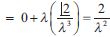 (using Gamma integral for positive integer)
Therefore Var(X ) = E(X2 )- E(X )2
= \(\frac { 2 }{ { \lambda }^{ 2 } } -\left( \frac { 1 }{ \lambda } \right) ^{ 2 }=\frac { 1 }{ { \lambda }^{ 2 } } \)
Hence the mean and variance are respectively \(\frac { 1 }{ \lambda } \) and \(\frac { 1 }{ { \lambda }^{ 2 } } \)
9.
Since f (x) is a probability density function, f (x) ≥ 0 and \(\int _{ -\infty }^{ \infty }{ f(x) } dx=1\)
That is \(\int _{ -\infty }^{ 1 }{ 0dx } +\int _{ 1 }^{ 5 }{ kdx } +\int _{ 5 }^{ \infty }{ 0dx } =1\)
\(0+k\left( x \right) _{ 1 }^{ 5 }+0=1\Rightarrow 4k=1\Rightarrow k=\frac { 1 }{ 4 } \)
Therefore the probability density function is
\(f\left( x \right) =\begin{cases} \begin{matrix} \frac { 1 }{ 4 } & 1\le x\le 5 \end{matrix} \\ \begin{matrix} 0 & Otherwise \end{matrix} \end{cases}\)
(i) Distribution function
The distribution function
\(F(x)=P\left( X\le x \right) =\int _{ -\infty }^{ x }{ f(u)dx } \)
When x < 1, \(F(x)=\int _{ -\infty }^{ x }{ f(u)du } =\int _{ -\infty }^{ x }{ oldu } =0\)
When 1 ≤ x ≤ 5 \(F(x)=\int _{ -\infty }^{ x }{ f(u)du=\int _{ -\infty }^{ x }{ 0du } +\int _{ 1 }^{ x }{ odu } +\int _{ 1 }^{ x }{ \frac { 1 }{ 4 } du } =\frac { 1 }{ 4 } (x-1) } \)
When x ≥ 5 \(F(x)=\int _{ -\infty }^{ x }{ f(u) } du=\int _{ -\infty }^{ x }{ odu } +\int _{ 1 }^{ 5 }{ \frac { 1 }{ 4 } du } +\int _{ 1 }^{ 5 }{ \frac { 1 }{ 4 } du } +\int _{ 5 }^{ 5 }{ odu } =1\)
Thus \(F(x)=\begin{cases} \begin{matrix} 0 & x<1 \end{matrix} \\ \begin{matrix} \frac { x-1 }{ 1 } & 1\le x\le 5 \end{matrix} \\ \begin{matrix} 1 & x>5 \end{matrix} \end{cases}\)
(ii) P(X < 3) = P(X ≤ 3) = F(3) = \(\frac { 3-1 }{ 2 } =\frac { 1 }{ 2 } \) (Since F(x) is continuous)
(iii) P(2 < X < 4) = P(2 ≤ X ≤ 4) F(4) - F(2) = \(\frac { 3 }{ 4 } -\frac { 1 }{ 4 } =\frac { 1 }{ 2 } \)
(iv) P(3 ≤ X ) = P(X ≥ 3) = 1− P(X < 3) = 1 - \(1-\frac { 1 }{ 2 } =\frac { 1 }{ 2 } \)
10.
Since the given function is a probability mass function, the total probability is one. That is \(\underset { x }{ \Sigma } f(x)=1\)
From the given data k + 2k + 6k + 5k + 6k +10k+1
\(30k=1\Rightarrow k=\frac { 1 }{ 30 } \)
Therefore the probability mass function is
| x | 1 | 2 | 3 | 4 | 5 | 6 |
| f(x) | \(\cfrac { 1 }{ 30 } \) | \(\cfrac { 2 }{ 30 } \) | \(\cfrac { 6 }{ 30 } \) | \(\cfrac { 5 }{ 30 } \) | \(\cfrac { 6 }{ 30 } \) | \(\cfrac { 10 }{ 30 } \) |
(i) P(2 < X < 6) = f(3)+ f(4)+ f(5) = \(\frac { 6 }{ 30 } +\frac { 5 }{ 30 } +\frac { 6 }{ 30 } =\frac { 17 }{ 30 } \)
(ii) P(2≤X≤5) = f(2)+f(3)+f(4) = \(\frac { 2 }{ 30 } +\frac { 6 }{ 30 } +\frac { 5 }{ 30 } =\frac { 13 }{ 30 } \)
(iii) P(2≤4) = f(1)+f(2)+f(3)+f(4) = \(\frac { 1 }{ 30 } +\frac { 2 }{ 30 } +\frac { 6 }{ 30 } +\frac { 5 }{ 30 } =\frac { 14 }{ 30 } \)
(iv) P(3>X) = f(4)+f(5)+f(6) = \(\frac { 5 }{ 30 } +\frac { 6 }{ 30 } +\frac { 10 }{ 30 } =\frac { 21 }{ 30 } \)
11.
By definition the cumulative distribution function for discrete random variable is
\(F(x)P\left( X\le x \right) =\underset { { x }_{ 1 }\le x }{ \Sigma } P(X={ x }_{ 1 })\)
\(P(X<1)=0\) for -∞
\(F(1)=P\left( X\le 1 \right) =\underset { { x }_{ 1 }\le x }{ \Sigma } P(X={ x }_{ i })=\sum _{ -\infty }^{ 1 }{ P(X=x) } =P\left( X<1 \right) +P\left( X=1 \right) =0+\frac { 1 }{ 12 } =\frac { 1 }{ 12 }\)
\(F(2)=P\left( X\le 2 \right) =\sum _{ -\infty }^{ 2 }{ P\left( X=x \right) } =P\left( X\le 1 \right) +P\left( X=1 \right) +P\left( X=2 \right)\)
= \(0+\frac { 1 }{ 12 } +\frac { 5 }{ 12 } =\frac { 1 }{ 2 }\)
\(F(3)=P\left( X\le 3 \right) =\sum _{ -\infty }^{ 3 }{ P(X=x) } =P\left( X<1 \right) +P\left( X=1 \right) +P\left( X=2 \right) +P\left( X=3 \right)\)
= \(0+\frac { 1 }{ 2 } +\frac { 5 }{ 12 } +\frac { 5 }{ 12 } =\frac { 11 }{ 12 }\)
\(F(4)=P\left( X\le 4 \right) =\sum _{ -\infty }^{ 4 }{ P\left( X=x \right) } =P\left( X=1 \right) +P\left( X=2 \right) +P\left( X=3 \right) +P(X=4)\)
= \(0+\frac { 1 }{ 12 } +\frac { 5 }{ 12 } +\frac { 5 }{ 12 } +\frac { 1 }{ 12 } =1\)
\(F(x)=\{0, \quad-\infty \ldots\)

(ii) \(P(X\le 3)=F(3)\frac { 11 }{ 12 }\)
(iii) \(P(X\ge 2)=1-P\left( X<2 \right) =1-P(X\le 1)=1-F(1)=1-\frac { 1 }{ 12 } =\frac { 11 }{ 12 }\)
12.
Let p be the probability of the useful life hours of a fluorescent light.
n = 12
P = 0.9
q = 1-p = 0.1
P(X= x)= nCx px qn-x, x = 0, 1,2, .., n
(i) Exactly 10
P(X = 10) = 12C10(0.9)10(1 - 0.9)2
= 12C10(0.9)10 (0.1)2
(ii) Atleast 11
P(X≥11) = R(X = 11) + P(X = 12)
= 12C11(0.9)11 (0.1)1 + 12C12(0.9)12(0.1)6
= 12C1 (0.9)11 (0.1) + (0.9)12
= 12(0.9)11 (0.1) + (0.9)12
= (0.9)11 ((12)(0.1) + 0.9)
= (0.9)11 (1.2 + 0.9)
= (0.9)11 (2.1)
(ii) Atleast 2 will not have a useful
P(X,10) = 1 -P(X > 10)
= 1 - [P(X = 11) + P(X = 12)]
= 1-(2.1) (0.9)11
13.
Given n = 12
P = 0.9
(i) P(X = 10) = 12C10(0.9)10(1 - 0.9)2
= 12C10(0.9)10 (0.1)2
(ii) P(X 2: 11) = R(X = 11) + P(X = 12)
= 12C11(0.9)11 (0.1) + 12C12(0.9)12(0.1)6
= 12C (0.9)11 (0.1) + (0.9)12
= 12(0.9)11 (0.1) + (0.9)12
= (0.9)11 ((12)(0.1) + 0.9)
= (0.9)11 (1.2 + 0.9) = (0.9)11 (2.1)
(iii) P( at least 2 will not have a useful life of atleast 600 hours) = 1 - P( atleast 11 will have a useful life of atleast 600 hours)
= 1 - P(X ≥11)
= 1-2.1 (0.9)11
14.
Given
\(f(x)=\begin{cases} \begin{matrix} { Ke }^{ \frac { -x }{ 3 } } & \begin{matrix} for & x>0 \end{matrix} \end{matrix} \\ \begin{matrix} 0 & \begin{matrix} for & x\le 0 \end{matrix} \end{matrix} \end{cases}\)
(i) Since f(x) is a probability density function
\(\int _{ -\infty }^{ \infty }{ f(x) } dx=1\)
\(\Rightarrow \int _{ 0 }^{ \infty }{ K.{ e }^{ \frac { -x }{ 3 } } } dx=1\Rightarrow k\frac { \left[ { e }^{ \frac { -x }{ 3 } } \right] ^{ \infty } }{ -\frac { 1 }{ 3 } } \)
\(\Rightarrow -3k\left[ { e }^{ -\infty }-{ e }^{ 0 } \right] =1\) [∵ e∞ = 0, e0 = 1]
\(\Rightarrow 3k=1\Rightarrow k=\frac { 1 }{ 3 } \)
\(\therefore k=\cfrac { 1 }{ 3 } \)
(ii) The distribution function F(x) = \(\int _{ -\infty }^{ x }{ f(u)du } \)
Case 1: x < 0,
\(F(x)=\int _{ -\infty }^{ x }{ f(x)dx=0 } \)
Case 2: x > 0,
\(f(x)=\int _{ -\infty }^{ x }{ f(x)dx } \)
= \(\int _{ -\infty }^{ 0 }{ f(x)dx+\int _{ 0 }^{ x }{ f(x) } dx } \)
= \(0+k\int _{ 0 }^{ x }{ { e }^{ \frac { -x }{ 3 } } } dx\)
= \(\frac { 1 }{ 3 } \left[ \cfrac { { e }^{ \frac { -x }{ 3 } } }{ -\frac { 1 }{ 3 } } \right] =-\left[ { e }^{ -\frac { x }{ 3 } }-{ e }^{ o } \right] \)
= \(-[{ e }^{ -\frac { x }{ 3 } }-1]\)
= \(1-{ e }^{ -\frac { x }{ 3 } }\)
\(\therefore F(x)=\begin{cases} \begin{matrix} 0 & x\le 0 \end{matrix} \\ \begin{matrix} 1-{ e }^{ \frac { -x }{ 3 } } & x>0 \end{matrix} \end{cases}\)
(iii) p(X < 3)
= \(\int _{ 0 }^{ 3 }{ ke^{ -\frac { x }{ 3 } } } dx=\cfrac { 1 }{ 3 } \int _{ 0 }^{ 3 }{ { e }^{ -\frac { x }{ 3 } }dx } \)
= \(\cfrac { 1 }{ 3 } \left[ \frac { { e }^{ -\frac { x }{ 3 } } }{ \frac { -1 }{ 3 } } \right] \)
= -[e-1-e0] = -[e-1-1]
(iv) \(p(5\le X)=p(X\ge 5)=\int _{ 5 }^{ \infty }{ f(x)dx } \)
= \(\int _{ 5 }^{ \infty }{ ke^{ -\frac { x }{ 3 } } } dx=\cfrac { 1 }{ 3 } \cfrac { \left[ { e }^{ -\frac { x }{ 3 } } \right] _{ 5 }^{ \infty } }{ \frac { -1 }{ 3 } } \)
= \(-\left[ { e }^{ -\infty }-e^{ \frac { -3 }{ 5 } } \right] =\left[ 0-{ e }^{ \frac { -5 }{ 3 } } \right] \)
= \({ e }^{ \frac { -5 }{ 3 } }\)
(v) \(p(X\le 4)=\int _{ -\infty }^{ 4 }{ f(x)dx } \)
= \(\int _{ -\infty }^{ 0 }{ f(x)dx+\int _{ 0 }^{ 4 }{ f(x)dx } } \)
= \(0+\int _{ 0 }^{ 4 }{ { ke }^{ -\frac { x }{ 3 } }dx } =k\left[ \frac { { e }^{ -\frac { x }{ 3 } } }{ -\frac { 1 }{ 3 } } \right] _{ 0 }^{ 4 }\)
= \(\cfrac { 1 }{ 3 } \cfrac { \left[ { e }^{ -\frac { x }{ 3 } } \right] _{ 0 }^{ 4 } }{ -\frac { 1 }{ 3 } } =-\left[ { e }^{ \frac { -4 }{ 3 } }-{ e }^{ o } \right] \)
= \(-\left[ { e }^{ \frac { -4 }{ 3 } }-1 \right] =1-{ e }^{ \frac { -4 }{ 3 } }\)
15.
Given \(p=\frac { 3 }{ 4 }\)
n = 5
P(X = x) = nCxpx (1-p)n-x
\(P(X=3)={ 5C }_{ 3 }\left( \frac { 3 }{ 4 } \right) ^{ 3 }\left( 1-\frac { 3 }{ 4 } \right) ^{ 2 }\)
\(P(X=3)={ 5C }_{ 2 }\left( \frac { 3 }{ 4 } \right) ^{ 3 }\left( \frac { 1 }{ 4 } \right) ^{ 2 }\) [∵nCr = nCn-r]
\(P(X=3)=\frac{5 \times 4}{2 \times 1} \times \frac{3 \times 3 \times 3}{4 \times 4 \times 4 \times 4 \times 4}\)
= \(\frac { 135 }{ 512 }\)
16.
\(\mathrm{n}=9, \mathrm{p}=\frac{1}{2}, \mathrm{k}=7
\)
\(
\mathrm{P}(X=x)={ }^{n} C_{x} p^{x} q^{n-x}, x=0,1,2, \ldots, n
\)
\(p =\frac{1}{2}
\)
\(q =1-p=\frac{1}{2} \)
\(P(X=7) ={ }^{9} C_{7}\left(\frac{1}{2}\right)^{7}\left(\frac{1}{2}\right)^{2}
\)
\( =\frac{9 \times 8}{2} \times \frac{1}{2^{9}} \)
\( =36 \times \frac{1}{512}=\frac{9}{128}
\)
17.
\(\)\(Mean=E(X)=\int _{ 1 }^{ 2 }{ f(x)dx=\int _{ 1 }^{ 2 }{ 2((x-1)dx } }\)
\(=2\left[\frac{8}{3}-\frac{4}{2}-\frac{1}{3}+\frac{1}{2}\right]\)
\(=2\left(\frac{7}{3}-\frac{3}{2}\right)\)
\(=2 \times \frac{5}{6}\)
\(=\frac{5}{3}\)
\(E({ x }^{ 2 })=\int _{ 1 }^{ 2 }{ { x }^{ 2 }f(x)dx }\)
= \(\int _{ 1 }^{ 2 }{ { x }^{ 2 }.2\left( x-1 \right) } dx\)
= \(2\int _{ 1 }^{ 2 }{ ({ x }^{ 3 }-{ x }^{ 2 })dx }\)
= \(2\left[ \frac { { x }^{ 4 } }{ 4 } -\frac { { x }^{ 3 } }{ 3 } \right] _{ 1 }^{ 2 }\)
= \(2\left[ \left( 4-\frac { 8 }{ 3 } \right) -\left( \frac { 1 }{ 4 } -\frac { 1 }{ 3 } \right) \right]\)
= \(2\left[ \frac { 4 }{ 3 } +\frac { 1 }{ 12 } \right] =2\left[ \frac { 16+1 }{ 12 } \right]\)
= \(\frac { 17 }{ 6 }\)
ஃ Var(X) = E(X2) - [E(X)]2
= \(\frac { 17 }{ 6 } -(\frac{5}{ 3 }^{ 2 })=\frac { 17 }{ 6 } -\frac { 25 }{ 9 }\)
= \(\frac{51-50}{18}\)
= \(\frac{1}{18}\)
18.
(c)
19.
(b)
1.56
20.
(b)
\(\frac { 11 }{ 16 } \)
21.
(c)
4 var (X)
22.
(d)
\(\frac { 5 }{ 4 } \)
23.
(a)
32
24.
(a)
0
25.
(b)
26.
(d)
0.96
27.
(b)
28.
(a)
1 and \(\frac { 1 }{ 2 } \)
29.
(d)
\(\left( \frac { 10 }{ 5 } \right) \left( \frac { 3 }{ 5 } \right) ^{ 5 }\left( \frac { 2 }{ 5 } \right) ^{ 5 }\)
30.
(a)
31.
(d)
32.
(d)
2

12th Standard Syllabus & Materials
12th Standard
TN 12th Computer Applications வலையமைப்பு வடமிடல் Sample Question Papers Study Material - QB365 Set A
NEW12th Standard
TN 12th Computer Applications களப்பெயர் முறைமை (DNS) Sample Question Papers Study Material - QB365 Set A
NEW12th Standard
TN 12th Computer Applications வலையமைப்பு எடுத்துக்காட்டுகள் மற்றும் நெறிமுறைகள் Sample Question Papers Study Material - QB365 Set A
NEW12th Standard
TN 12th Computer Applications கணினி வலையமைப்பு ஓர் அறிமுகம் Sample Question Papers Study Material - QB365 Set A



Tamilnadu Stateboard 12th Standard Subjects
Maths

Chemistry

Physics

Biology

Computer Science

Business Maths and Statistics

Economics

Commerce

Accountancy

History

Computer Applications
Biology
Computer Technology
Computer Applications
Computer Science
Business Maths and Statistics
Commerce
Economics
Maths
Chemistry
Physics
Computer Technology
History
Accountancy

Tamil

English

French
Tamilnadu Stateboard Standards

