
 100% FREE ACCESS
12th Standard Syllabus & Materials
12th Standard
TN 12th Computer Applications மின்னணு தரவு பரிமாற்றம் Sample Question Papers Study Material - QB365 Set A
NEW12th Standard
TN 12th Computer Applications மின் - வணிக பாதுகாப்பு அமைப்புகள் Sample Question Papers Study Material - QB365 Set A
NEW12th Standard
TN 12th Computer Applications மின்னணு செலுத்தல் முறைகள் Sample Question Papers Study Material - QB365 Set A
NEW12th Standard
TN 12th Computer Applications மின் - வணிகம் Sample Question Papers Study Material - QB365 Set A
NEW12th Standard
TN 12th Computer Applications திறந்த மூல கருத்துருக்கள் Sample Question Papers Study Material - QB365 Set A
NEW12th Standard
TN 12th Computer Applications வலையமைப்பு வடமிடல் Sample Question Papers Study Material - QB365 Set A

Published on: 02/09/2022
QB365 provides a detailed and simple solution for every Possible Creative Questions in Class 12 Physics Subject - Retirement and Death of a Partner, English Medium. It will help Students to get more practice questions, Students can Practice these question papers in addition to score best marks.
Download Tamil Nadu 12th Standard Physics question papers, model tests, one-mark questions, important questions, and public exam papers in PDF format. Free study materials and answer keys for TN State Board students.
Questions + Answers key
Take MCQ Physics Test1.
The instantaneous current and voltage of an a.c circuit are given by i = 10 sin 314t A and V = 50 sin (314t + π/2)V. What is the power dissipation in the circuit?
2.
In a LCR circuit, the voltage across an inductor, capacitor and resistance are 10V, 10V and 30V respectively, what is the phase difference between the applied voltage and the current in the circuit?
3.
In an a.c circuit R = 4Ω; z = 5Ω, Vrms = 200V and Irms = 1.5A calculate the average power consumed over a full cycle.
4.
Explain how power can be transmitted efficiently to long distance.
5.
Explain the mutual induction between two long solenoids. Obtain an expression for the mutual inductance.
6.
Obtain an expression for angular frequency of LC oscillations?
7.
Write the analogies between electrical and mechanical quantities
8.
Explain the mechanical analogy of LC oscillations by quantitative treatment.
9.
Straight in LC oscillations, the sum of energies stored in capacitor & the inductors is constant in time.
10.
Define Power in AC circuits? Derive an relation between true power & virtual power?
11.
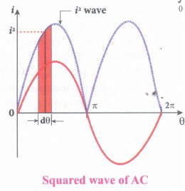
Define RMS value of AC. Derive a relation between RMS value of AC voltage & maximum voltage.
12.
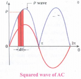
Derive an expression for the RMS value of AC.
13.
Derive a relation between mean or average value of AC and its peak value.
14.
Show that the total energy is constant druing LC oscillations.
15.
Using Faraday’s law of electromagnetic induction, derive an equation for motional emf.
1.
Phase difference between V and i = \(\frac{\pi}{2}\)red
∴ Paverage = \(\frac { { V }_{ m }{ I }_{ m } }{ 2 } \). cos Φ = \(\frac { 50\times 10 }{ 2 } \) cos 0o
2.
Given: Voltage across an inductor
VL=10V
Voltage across a capacitor Vc = 10V
Voltage across resistance Ve = 30
The phase difference between applied voltage and
Solution:
current in the circuit tan Φ = \(\frac { { V }_{ L }-{ V }_{ C } }{ { V }_{ R } } \)
tan Φ = \(\frac { 10-10 }{ 30 } \)
tan Φ = 0
∴ phase difference Φ = 0
3.
P Average = Vrms. Irms. cost
= Vrms. Irms. \(\frac{R}{z}\)
= 200 x 1.5 x \(\frac45\)
Paverage = 240W.
4.
(i) The electric power generated in a power station situated in a remote place is transmitted to different regions for domestic and industrial use.
(ii) For long-distance transmission, power lines are made of conducting material like aluminum. There is always some power loss associated with these lines.
(iii) If I is the current through the wire and R the resistance, a considerable amount of electric power FR is dissipated as heat. Hence, the power at the receiving end will be much lesser than the actual power generated.
(iv) However, by transmitting the electrical energy at a higher voltage, the power loss can be controlled as is evident from the following two cases
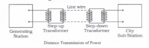
Case (1) A power of 11,000 W is transmitted at 220 V.
Power P = VI
I = \(\frac{P}{V}=\frac{11,000}{220}\) = 0.5A
If R is the resistance of line wires,
Power loss = I2R = 502R = 2500(R) watts.
Case (2) 11,000 W power is transmitted at 22,000 V.
I = \(\frac{P}{V}=\frac{11,000}{22,000}\)= 0.5A
Power loss = I2R = (0.5)2R = 0.25(R) watts. Hence it is evident that if power is transmitted at a higher voltage the loss of energy in the form of heat can be considerably reduced.
5.
(i) S1 and S2 are two long solenoids each length l. The solenoid S2 is wound closely over the solenoid S1.
(ii) N1 and N2 are the number of turns in the solenoids S1 and S2 respectively. Both the solenoids are considered to have the same area of cross-section A as they are closely wound together.
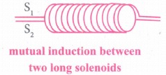
(iii) I1 is the current flowing through the solenoid S1 The magnetic field B1 produced at any point inside the solenoid S1 due to the current I1 is
\({ B }_{ 1 }={ \mu }_{ o }\frac { { N }_{ i } }{ l } { I }_{ 1 }\) ...(1)
(iv) The magnetic flux linked with each turn of S2 is equal to B1A.
Total magnetic flux linked with solenoid S2 having N2 turns is
Φ2 = \(\frac { { \mu }_{ o }{ N }_{ 1 }N_{ 2 }{ AI }_{ 1 } }{ l } \) ...(2)
But Φ2 = MI1 ...(3)
where M is the coefficient of mutual induction between S1 and S2
From equations (2) and (3),
MI1 = \(\frac { { \mu }_{ o }{ N }_{ 1 }N_{ 2 }{ AI }_{ 1 } }{ l } \); M = \(\frac { { \mu }_{ o }{ N }_{ 1 }N_{ 2 }A }{ l } \)
(v) If the core is filled with a magnetic material of permeability μ,
M = \(\frac { { \mu }_{ o }{ N }_{ 1 }N_{ 2 }A }{ l } \)
6.
By differentiating equation twice, we get
q(t) Qm cos(ωt + Φ) ...(1)
\(\frac { { d }^{ 2 }q }{ { dt }^{ 2 } } \) = - Qm ω2 cos (ωt + Φ) ...(2)
Substituting equations (1) and (2) in equation
\(\frac { dU }{ dt } =\frac { 1 }{ 2 } L\left( 2i\frac { di }{ dt } \right) +\frac { 1 }{ 2C } \left( 2q\frac { dq }{ dt } \right) =0\)
(or) \(L\frac { { d }^{ 2 }q }{ { dt }^{ 2 } } +\frac { 1 }{ C } q=0\)
we obtain
L[- Qm ω2 cos (ωt + Φ)] + \(\frac { 1 }{ C } \) Qm cos (ωt + Φ) = 0
Rearranging the terms, the angular frequency of LC oscillations is given by
ω = \(\frac { 1 }{ \sqrt { LC } } \)
This equation is the same as that obtained from qualitative analogy.
7.
|
Electrical system |
Mechanical system |
|---|---|
| Charge q | Displacement x |
| Current i = \(\frac { dq }{ dt } \) | Velocity v = \(\frac { dx }{ dt } \) |
| Inductance L | Mass m |
| Reciprocal of capacitance \(\frac { 1 }{ C } \) | Force constant k |
| Electrical energy = \(\frac { 1 }{ 2 } \left( \frac { 1 }{ C } \right) { q }^{ 2 }\) | Potential energy = \(\frac { 1 }{ 2 } k{ x }^{ 2 }\) |
| Magnetic energy = \(\frac { 1 }{ 2 } \) Li2 | Kinetic energy = \(\frac { 1 }{ 2 } \) mv2 |
| Electromagnetic energy = \(U=\frac { 1 }{ 2 } \left( \frac { 1 }{ C } \right) { q }^{ 2 }\) + \(\frac12\)Li2 | Mechanic energy E = \(\frac { 1 }{ 2 } k{ x }^{ 2 }\) + \(\frac { 1 }{ 2 } \) mv2 |
8.
(i) The energy E remains constant for varying values of x and v. Differentiating E with respect to time, we get \(\frac { dE }{ dt } =\frac { 1 }{ 2 } \left( 2v\frac { dv }{ dt } \right) +\frac { 1 }{ 2 } k\left( \frac { dx }{ dt } \right) =0\)
or m \(\frac { { d }^{ 2 }x }{ { dt }^{ 2 } } +kx=0\)
since \(\frac { dx }{ dt } =\nu \) and \(\frac { dv }{ dt } =\frac { { d }^{ 2 }x }{ d{ t }^{ 2 } } \)
(ii) This is the differential equation of the oscillations of the spring-mass system. The general solution of an equation is of the form
x(t) = Xm cos (ωt + Φ)
where X is the maximum value of x(t), ω the angular frequency, and Φ the phase constant.
(iii) Similarly, the electromagnetic energy of the LC system is given by
\(U=\frac { 1 }{ 2 } { Li }^{ 2 }+\frac { 1 }{ 2 } \left( \frac { 1 }{ C } \right) { q }^{ 2 }\) = constant
Differentiating U with respect to time, we get
\(\frac { dU }{ dt } =\frac { 1 }{ 2 } L\left( 2i\frac { di }{ dt } \right) +\frac { 1 }{ 2C } \left( 2q\frac { dq }{ dt } \right) =0\)
(or) \(\frac { { d }^{ 2 }q }{ { dt }^{ 2 } } +\frac { 1 }{ C } q=0\) ....(1)
since \(i=\frac { dq }{ dt } \frac { di }{ dt } =\frac { { d }^{ 2 }q }{ d{ t }^{ 2 } } \)
(iv) The general solution of equation (1) is of the form
q(t) = Qm cos (ωt + Φ)
(v) where Qm is the maximum value of q(t), ω the angular frequency, and Φ the phase constant.
9.
(i) During LC oscillations in LC circuits, the energy of the system oscillates between the electric field of the capacitor and the magnetic field of the inductor.
(ii) Although these two forms of energy vary with time, the total energy remains constant. It means that LC oscillations take place in accordance with the law of conservation of energy.
Total energy, U= UE + UB = \(\frac { { q }^{ 2 } }{ 2C } +\frac { 1 }{ 2 } { Li }^{ 2 }\)
(iii) consider 3 different stages of LC oscillations and calculate the total energy of the system.
Case (i) When the charge in the capacitor, q Qm = and the current through the inductor, i = 0, the total energy is given by
\(U=\frac { { { Q }_{ m } }^{ 2 } }{ 2C } +0=\frac { { { Q }_{ m } }^{ 2 } }{ 2C } \)
The total energy is wholly electrical
Case (ii) When charge = 0; current = Im, the total energy is
\(U=0+\frac { 1 }{ 2 } { { Li }^{ 2 } }_{ m }=\frac { 1 }{ 2 } { { Li }^{ 2 } }_{ m }\)
\(=\frac { L }{ 2 } \times \left( \frac { { { Q }_{ m } }^{ 2 } }{ LC } \right) { Q }_{ m }\omega =\frac { { Q }_{ m } }{ \sqrt { LC } } \)
= \(\frac { { { Q }_{ m } }^{ 2 } }{ 2C } \)
Case (ii) When charge = 0 ; current = Im the total energy is
\(U=0+\frac { 1 }{ 2 } { { Li }^{ 2 } }_{ m }=\frac { 1 }{ 2 } { { Li }^{ 2 } }_{ m }\)
\(=\frac { L }{ 2 } \times \left( \frac { { { Q }_{ m } }^{ 2 } }{ LC } \right) \) since Im= \({ Q }_{ m }\omega =\frac { { Q }_{ m } }{ \sqrt { LC } } \)
= \(\frac { { { Q }_{ m } }^{ 2 } }{ 2C } \)
Case (iii) When charge = q; current = t. the total energy is
U = \(\frac { { q }^{ 2 } }{ 2C } +\frac { 1 }{ 2 } { Li }^{ 2 }\)
(iv) Since q = Qm = cos ωt, i = \(\frac { dq }{ dt } ={ Q }_{ m }=\omega \) sin ωt. The negative sign in current indicates that the charge in the capacitor decreases with time.
\(U=\frac { { { Q }_{ m } }^{ 2 }{ cos }^{ 2 }\omega t }{ 2C } +\frac { { { L{ \omega }^{ 2 }Q }_{ m } }^{ 2 }{ sin }^{ 2 }\omega t }{ 2 } \)
\(U=\frac { { { Q }_{ m } }^{ 2 }{ cos }^{ 2 }\omega t }{ 2C } +\frac { { { L{ \omega }^{ 2 }Q }_{ m } }^{ 2 }{ sin }^{ 2 }\omega t }{ 2LC } \)
since \({ \omega }^{ 2 }=\frac { 1 }{ LC } \)
= \(\frac { { { Q }_{ m } }^{ 2 } }{ 2C } { (cos }^{ 2 }\omega t+{ sin }^{ 2 }\omega t)\)
\(U=\frac { { { Q }_{ m } }^{ 2 } }{ 2C } \)
From the above three cases, it is clear that the total energy of the system remains constant.
10.
(i) Power of a circuit is defined as the rate of consumption of electric energy in that circuit. It is given by the product of the voltage and current. In an AC circuit, the voltage and current vary continuously with time.
(ii) The alternating voltage and alternating current in the series RLC circuit at an instant are given by
v = Vm sin ωt and i = Im sin(ωt + Φ)
(iii) Where Φ is is the phase angle between v and i. The instantaneous power is then written as
P = vi
= VmIm sin ω sin(ωt + Φ)
= VmImsin ωt[sin ωt cos Φ - cos ωt sin Φ)
P = VmIm[cos Φ sin2 ωt - sin ωt cos ωt sin Φ]
(iv) Here the average of sin2ωt over a cycle is \(\frac { 1 }{ 2 } \) and that of sin wt cos wt is zero. Substituting these values, we obtain average power over a cycle.
= \(\frac { { V }_{ m } }{ \sqrt { 2 } } \frac { { I }_{ m } }{ \sqrt { 2 } } \) cos Φ
Pav = VRMSIRMS cosΦ
(v) where VRMS IRMS is called apparent power and cos Φ is power factor. The average power of an AC circuit is also known as the true power of the circuit.
11.
(i) RMS value is also defined as that value of the steady current which when flowing through a given circuit for a given time produces the same amount of heat as produced by the alternating current when flowing through the same circuit for the same time. The effective value of an alternating voltage is represented by Veff
(ii) The alternating current i = Im sin ωt or i = Im sin θ, is represented graphically in Figure. The corresponding squared current wave is also shown by the dotted lines.
(iii) The sum of the squares of all currents over one cycle is given by the area of one cycle of squared wave. Therefore,
IRMS = \(\sqrt{\frac{Area \ of \ one \ cycle \ of \ squared \ wave}{Base\ length \ of \ one\ cycle}}\) ...(1)
(iv) An elementary area of thickness dθ is considered in the first half-cycle of the squared current wave as shown in Figure. Let e be the mid-ordinate of the element. Area of the element = l2dθ
Area of one cycle of squared
wave = \(\int _{ 0 }^{ 2\pi }{ { i }^{ 2 }d\theta } \)
= \(\int _{ 0 }^{ 2\pi }{ { { I }^{ 2 } }_{ m } } { sin }^{ 2 }\theta d\theta ={ { I }^{ 2 } }_{ m }\int _{ 0 }^{ 2\pi }{ { sin }^{ 2 }\theta d\theta } \)
\(={ { I }^{ 2 } }_{ m }\int _{ 0 }^{ 2\pi }{ \left[ \frac { 1-cos2\theta }{ 2 } \right] d\theta } \)
since \({ sin }^{ 2 }\theta =\frac { 1-cos2\theta }{ 2 } \)
= \(\frac { { { I }^{ 2 } }_{ m } }{ 2 } \left[ \int _{ 0 }^{ \pi }{ id\theta } =\int _{ 0 }^{ \pi }{ { I }_{ m }cos2\theta d\theta } \right] \)
= \(\frac { { { I }^{ 2 } }_{ m } }{ 2 } { \left[ \theta -\frac { sin2\theta }{ 2 } \right] }_{ 0 }^{ 2\pi }\)
= \(\frac { { { I }^{ 2 } }_{ m } }{ 2 } \left[ \left( 2\pi -\frac { sin2\times 2\pi }{ 2 } \right) -\left( 0-\frac { sin0 }{ 2 } \right) \right] \)
= \(\frac { { { I }^{ 2 } }_{ m } }{ 2 } \)x2π = I2m π [∵ sin 0 = sin 4π = 0]
Substituting this in equation'(1), we get
\(\sqrt { \frac { { { I }^{ 2 } }_{ m }\pi }{ 2\pi } } =\frac { { { I }^{ 2 } }_{ m } }{ \sqrt { 2 } } \)
[Base length of cone cycle is 2π]
IRMS = 0.707 Im
Thus we find that for a symmetrical sinusoidal current RMS value of current is 70.7 % of its peak value. Similarly for alternating voltage, it can be shown that
Vrms = 0.707 Im
12.
(i) The term RMS refers to time-varying sinusoidal currents and voltages and is not used in DC systems.
(ii) The root mean square value of an alternating current is defined as the square root of the mean of the squares of all currents over one cycle. It is denoted by IRMS. For alternating voltages, the RMS value is given by IVRM.
(iii) The alternating current i = Im sin ωt or i = Im sin θ, is represented graphically in Figure. The corresponding squared current wave is also shown by the dotted lines.
(iv) The sum of the squares of all currents over one cycle is given by the area of one cycle of the squared wave. Therefore,
IRMS = \(\sqrt{\frac{Area \ of \ one \ cycle \ of \ squared \ wave}{Base\ length \ of \ one\ cycle}}\) ....(1)
(v) An elementary area of thickness dθ is considered in the first half-cycle of the squared current wave as shown in Figure. Let i2 be the mid-ordinate of the element. Area of the element = i2dθ
Area of one cycle of squared.
wave = \(\int _{ 0 }^{ 2\pi }{ { i }^{ 2 }d\theta } \)
= \(\int _{ 0 }^{ 2\pi }{ { { I }^{ 2 } }_{ m } } { sin }^{ 2 }\theta d\theta ={ { I }^{ 2 } }_{ m }\int _{ 0 }^{ 2\pi }{ { sin }^{ 2 }\theta d\theta } \)
= \({ { I }^{ 2 } }_{ m }\int _{ 0 }^{ 2\pi }{ \left[ \frac { 1-cos2\theta }{ 2 } \right] d\theta } \)
since \({ sin }^{ 2 }\theta =\frac { 1-cos2\theta }{ 2 } \)
= \(\frac { { { I }^{ 2 } }_{ m } }{ 2 } \left[ \int _{ 0 }^{ \pi }{ id\theta } =\int _{ 0 }^{ \pi }{ { I }_{ m }cos2\theta d\theta } \right] \)
= \(\frac { { { I }^{ 2 } }_{ m } }{ 2 } { \left[ \theta -\frac { sin2\theta }{ 2 } \right] }_{ 0 }^{ 2\pi }\)
= \(\frac { { { I }^{ 2 } }_{ m } }{ 2 } \left[ \left( 2\pi -\frac { sin2\times 2\pi }{ 2 } \right) -\left( 0-\frac { sin0 }{ 2 } \right) \right] \)
= \(\frac { { { I }^{ 2 } }_{ m } }{ 2 } \times \pi ={ { I }^{ 2 } }_{ m }\pi \) [∵ sin 0 = sin 4π = 0]
Substituting this in equation (1), we get
\(\sqrt { \frac { { { I }^{ 2 } }_{ m }\pi }{ 2\pi } } =\frac { { { I }^{ 2 } }_{ m } }{ \sqrt { 2 } } \) [Base length of cone cycle is 2π]
IRMS = 0.707 Im
13.
(i) The magnitude of an alternating current in a circuit changes from one instant to other instant and its direction also reverses for every half cycle.
(ii) During positive half cycle, current is taken as positive and during negative cycle it is negative. Therefore mean or average value of symmetrical alternating current over one complete cycle is zero.
(iii) Therefore the average or mean value is measured over one half of a cycle. These electrical terms, average current and average voltage can be used in both AC and DC circuit analysis and calculations.
(iv) The average value of alternating current is defined as the average of all values of current over a positive half-cycle or negative half-cycle.
(v) The instantaneous value of sinusoidal alternating current is given by the equation
i = Im sin ωt or i = Im sinθ (where θ = ωt) whose graphical representation is given in Figure.
(vi) The sum of all currents over a half-cycle is given by area of positive half-cycle (or negative half-cycle). Therefore,
Iav = \(\frac{Area \ of \ positive \ half-cycle (or \ negative \ half -cycle)}{Base \ lenght \ of \ half - cycle)}\) ...(1)
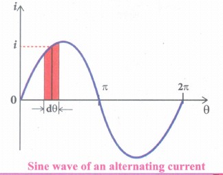
(vii) Consider an elementary strip of thickness dθ in the positive half-cycle of the current wave. Let i be the mid-ordinate of that strip.
Area of the elementary strip = i dθ
Area of positive half-cycle
= \(\int _{ 0 }^{ \pi }{ id\theta } =\int _{ 0 }^{ \pi }{ { I }_{ m }sin\theta d\theta } \)
= \({ I }_{ m }{ [-cos\theta ] }_{ 0 }^{ \pi }={ -I }_{ m }[cos\pi -cos0]=2{ I }_{ m }\)
Substituting this in equation (1), we get (The base length of half-cycle is π)
Average value of AC, Iav = \(\frac { { 2I }_{ m } }{ \pi } \)
Iav = 0.637 Im
(viii) Hence the average value of AC is 0.637 times the maximum value Im of the alternating current. For negative half cycle, Iav = -0.637 Im
14.
(i) During LC oscillations in LC circuits, the energy of the system oscillates between the electric field of the capacitor and the magnetic field of the inductor. Although these two forms of energy vary with time, the total energy remains constant. It means that LC oscillations take place in accordance with the law of conservation of energy.
Total energy, \(U={ U }_{ E }+{ U }_{ B }=\cfrac { { q }^{ 2 } }{ 2C } +\cfrac { 1 }{ 2 } { Li }^{ 2 }\)
(ii) Let us consider 3 different stages of LC oscillations and calculate the total energy of the system. Case (i) When the charge in the capacitor, q = Qm and the current through the inductor, i = 0, the total energy is given by
\(U=\cfrac { { Q }_{ m }^{ 2 } }{ 2C } +0=\cfrac { { Q }_{ m }^{ 2 } }{ 2C } \)
The total energy is wholly electrical.
Case (ii) When charge = 0 ; current = Im ' the total energy is
\(U=0+\cfrac { { Q }_{ m }^{ 2 } }{ 2C } { LI }_{ 3 }^{ 2 }=\cfrac { 1 }{ 2 } { LI }_{ m }^{ 2 }\)
= \(\cfrac { 1 }{ 2 } \times \left( \cfrac { { Q }_{ m }^{ 2 } }{ LC } \right) Since\quad { I }_{ m }={ Q }_{ m }\omega =\cfrac { { Q }_{ m } }{ \sqrt { LC } } \)
= \(\cfrac { { Q }_{ m }^{ 2 } }{ LC } \)
The total energy is wholly magnetic.
Case (iii) When charge = q; current = i, the total energy is
\(U=\cfrac { { q }^{ 2 } }{ 2C } +\cfrac { 1 }{ 2 } { Li }^{ 2 }\)
Since \(q={ Q }_{ m }\)
\(i=-\cfrac { dq }{ dt } ={ Q }_{ m }\)
The negative sign in current indicates that the charge in the capacitor decreases with time
\(U=\cfrac { { Q }_{ m }^{ 2 }{ cos }^{ 2 }\omega t }{ 2C } +\cfrac { { L\omega }^{ 2 }{ Q }_{ m }^{ 2 }\omega t }{ 2 } \)
= \(U=\cfrac { { Q }_{ m }^{ 2 }{ cos }^{ 2 }\omega t }{ 2C } +\cfrac { { L\omega }^{ 2 }{ Q }_{ m }^{ 2 }\omega t }{ 2 } \)
= \(\cfrac { { Q }_{ m }^{ 2 } }{ 2C } \left( { cos }^{ 2 }+\omega t+{ sin }^{ 2 }\omega t \right) \)
\(U=\cfrac { { Q }_{ m }^{ 2 } }{ 2C } \)
From above three cases, it is clear that the total energy of the system remains constant.
15.
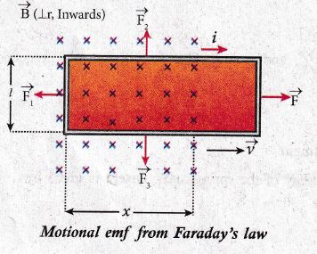
(i) Consider a rectangular conducting loop of width 1 in a uniform magnetic field \(\vec { B } \) which is perpendicular to the plane of the loop and is directed inwards.
(ii) A part of the loop is in the magnetic field while the remaining part is outside the loop as shown in Figure.
(iii) When the loop is pulled with a constant velocity \(\vec { v } \) to the right, the area of the portion of the loop within the magnetic field will decrease.
(iv) Thus, the flux linked with the loop will also decrease. According to Faraday's law, an electric current is induced in the loop which flows in a direction so as to oppose the pull of the loop.
(v) Let x be the length of the loop which is still within the magnetic field, then its area is lx. The magnetic flux linked with the loop is
\({ \phi }_{ B }=\int _{ A }^{ }{ B.d } \vec { A } =BAcos\theta \)
Here θ = 0o and cos 0o = 1
= BA
\({ \phi }_{ B }=Blx\)
(vi) As this magnetic flux decreases due to the movement of the loop, the magnitude of the induced emf is given by
\(\varepsilon =\frac { d{ \Phi }_{ B } }{ dt } =\frac { d }{ dt } (Blx)\)
(vii) Here, both B and 1 are constants. Therefore,
\(\varepsilon =Bl\frac { dx }{ dt } \)
ε = Blv
where \(v=\frac { dx }{ dt } \) is the velocity of the loop. This emf is known as motional emf since it is produced due to the movement of the loop in the magnetic field.

12th Standard Syllabus & Materials
12th Standard
TN 12th Computer Applications களப்பெயர் முறைமை (DNS) Sample Question Papers Study Material - QB365 Set A
NEW12th Standard
TN 12th Computer Applications வலையமைப்பு எடுத்துக்காட்டுகள் மற்றும் நெறிமுறைகள் Sample Question Papers Study Material - QB365 Set A
NEW12th Standard
TN 12th Computer Applications கணினி வலையமைப்பு ஓர் அறிமுகம் Sample Question Papers Study Material - QB365 Set A
NEW12th Standard
TN 12th Computer Applications PHP-உடன் MySQL-ஐ இணைத்தல் Sample Question Papers Study Material - QB365 Set A



Tamilnadu Stateboard 12th Standard Subjects

Maths

Chemistry
Physics

Biology

Computer Science

Business Maths and Statistics

Economics

Commerce

Accountancy

History

Computer Applications
Biology
Computer Technology
Computer Applications
Computer Science
Business Maths and Statistics
Commerce
Economics
Maths
Chemistry
Physics
Computer Technology
History
Accountancy

Tamil

English

French
Tamilnadu Stateboard Standards

