
 100% FREE ACCESS
12th Standard Syllabus & Materials
12th Standard
TN 12th Computer Applications மின்னணு தரவு பரிமாற்றம் Sample Question Papers Study Material - QB365 Set A
NEW12th Standard
TN 12th Computer Applications மின் - வணிக பாதுகாப்பு அமைப்புகள் Sample Question Papers Study Material - QB365 Set A
NEW12th Standard
TN 12th Computer Applications மின்னணு செலுத்தல் முறைகள் Sample Question Papers Study Material - QB365 Set A
NEW12th Standard
TN 12th Computer Applications மின் - வணிகம் Sample Question Papers Study Material - QB365 Set A
NEW12th Standard
TN 12th Computer Applications திறந்த மூல கருத்துருக்கள் Sample Question Papers Study Material - QB365 Set A
NEW12th Standard
TN 12th Computer Applications வலையமைப்பு வடமிடல் Sample Question Papers Study Material - QB365 Set A

Published on: 01/09/2022
QB365 provides a detailed and simple solution for every Possible Book Back Questions in Class 12 Physics Subject - Electrostatics, English Medium. It will help Students to get more practice questions, Students can Practice these question papers in addition to score best marks.
Download Tamil Nadu 12th Standard Physics question papers, model tests, one-mark questions, important questions, and public exam papers in PDF format. Free study materials and answer keys for TN State Board students.
Questions + Answers key
Take MCQ Physics Test1.
An electron and a proton are allowed to fall through the separation between the plates of a parallel plate capacitor of voltage 5 V and separation distance h = 1 mm as shown in the figure.
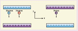
(a) Calculate the time of flight for both electron and proton
(b) Suppose if a neutron is allowed to fall, what is the time of flight?
(c) Among the three, which one will reach the bottom first? (Take mp = 1.6 x 10⁻²⁷ kg, me = 9.1 x 10⁻³¹ kg and g = 10 m s-2)
2.
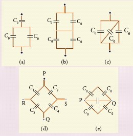
Calculate the resultant capacitances for each of the following combinations of capacitors.
3.
A spark plug in a bike or a car is used to ignite the air-fuel mixture in the engine. It consists of two electrodes separated by a gap of around 0.6 mm gap as shown in the figure.
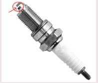
To create the spark, an electric field of magnitude 3 x 10⁶ Vm-1 is required.
(a) What potential difference must be applied to produce the spark?
(b) If the gap is increased, does the potential difference increase, decrease or remains the same?
(c) find the potential difference if the gap is 1 mm.
4.
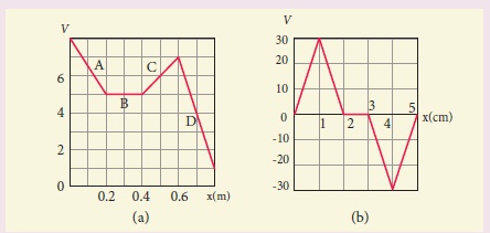
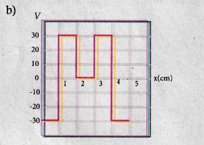
The electrostatic potential is given as a function of x in figure (i) and (ii). (a) Calculate the corresponding electric fields in regions A, B, C and D for the Figure (i). (b) Plot the electric field as a function of x for the figure (ii).
5.
Suppose a charge +q on Earth’s surface and another +q charge is placed on the surface of the Moon.
(a) Calculate the value of q required to balance the gravitational attraction between Earth and Moon.
(b) Suppose the distance between the Moon and Earth is halved, would the charge q change?
(Take mE = 5.9 x 1024 kg, mM = 7.9 x 10²² kg)
6.
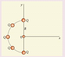
Five identical charges Q are placed equidistant on a semicircle as shown in the figure. Another point charge q is kept at the center of the circle of radius R. Calculate the electrostatic force experienced by the charge q.
7.
Two conducting spheres of radius r1 = 8 cm and r2 = 2 cm are separated by a distance much larger than 8 cm and are connected by a thin conducting wire as shown in the figure. A total charge of Q = +100 nC is placed on one of the spheres. After a fraction of a second, the charge Q is redistributed and both the spheres attain electrostatic equilibrium.
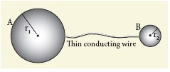
(a) Calculate the charge and surface charge density on each sphere.
(b) Calculate the potential at the surface of each sphere.
8.
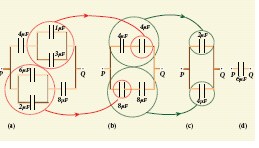
Find the equivalent capacitance between P and Q for the configuration shown below in the figure (a).
9.
A parallel plate capacitor filled with mica having εr = 5 is connected to a 10 V battery. The area of the parallel plate is 6 cm2 and separation distance is 6 mm.
(a) Find the capacitance and stored charge.
(b) After the capacitor is fully charged, the battery is disconnected and the dielectric is removed carefully.
Calculate the new values of capacitance, stored energy and charge.
10.
11.
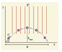
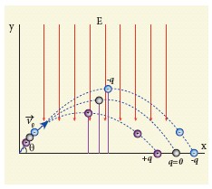
A small ball of conducting material having a charge +q and mass m is thrown upward at an angle θ to horizontal surface with an initial speed vo as shown in the figure. There exists an uniform electric field E downward along with the gravitational field g. Calculate the range, maximum height and time of flight in the motion of this charged ball. Neglect the effect of air and treat the ball as a point mass.
12.
(a) Calculate the electric potential at points P and Q as shown in the figure below.
(b) Suppose the charge + 9μC is replaced by - 9 μC find the electrostatic potentials at points P and Q.
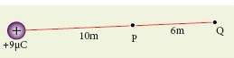
(c) Calculate the work done to bring a test charge +2 μC from infinity to the point Q. Assume the charge +9 μC is held fixed at origin and +2 μC is brought from infinity to P.
13.
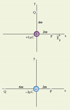
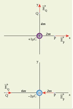
Calculate the electric field at points P, Q for the following two cases, as shown in the figure.
(a) A positive point charge +1 μC is placed at the origin.
(b) A negative point charge -2 μC is placed at the origin.
14.
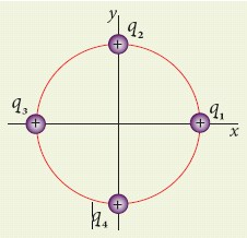
Consider four equal charges q1, q2, q3 and q4 = q = +1 μC located at four different points on a circle of radius 1m, as shown in the figure. Calculate the total force acting on the charge q1 due to all the other charges.
15.
Calculate the electrostatic force and gravitational force between the proton and the electron in a hydrogen atom. They are separated by a distance of 5.3 x 10⁻¹¹ m. The magnitude of charges on the electron and proton are 1.6 x 10⁻¹⁹ C. Mass of the electron is me = 9.1 x 10⁻³¹ kg and mass of proton is mp = 1.6 x 10⁻²⁷ kg.
16.
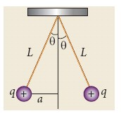
Two small-sized identical equally charged spheres, each having mass 1 g are hanging in equilibrium as shown in the figure. The length of each string is 10 cm and the angle θ is 30° with the vertical. Calculate the magnitude of the charge in each sphere. (Take g = 10 ms−2)
17.
Consider two point charges q1 and q2 at rest as shown in the figure.
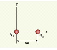
They are separated by a distance of 1m. Calculate the force experienced by the two charges for the following cases:
(a) q1 = +2μC and q2 = +3μC
(b) q1 = +2μC and q2 = -3μC
(c) q1= +2μC and q2 = -3μC kept in water (εr = 80)
18.
1.
h = 1 x 10⁻³ m, e = 1.6 x 10⁻¹⁹ C, me = 9.1 x 10⁻³¹ kg, mp =1.6 x 10⁻²⁷ kg
(a) (i) Time of flight for electron \(t_{c}=\sqrt{\frac{2 h m_{e}}{e E}}\)
Where,
\(E =\frac{V}{d}=\frac{5}{1 \times 10^{-3}}=5000 \mathrm{Vm}^{-1} \)
\(t_{e} =\sqrt{\frac{2 \times 1 \times 10^{-3} \times 9.1 \times 10^{-31}}{1.6 \times 10^{-19} \times 5000}}=\sqrt{\frac{18.2 \times 10^{-34}}{8 \times 10^{-16}}}=\sqrt{2.275 \times 10^{-18}} \)
= 1.5 x 10⁻⁹s
te = 1.5 ns (ignoring the gravity)
(ii) Time of flight for proton \(t_{p}=\sqrt{\frac{2 h m_{p}}{e E}}\)
\(t_{p} =\sqrt{\frac{2 \times 1 \times 10^{-3} \times 1.6 \times 10^{-27}}{1.6 \times 10^{-19} \times 5000}} \)
\(=\sqrt{\frac{3.2 \times 10^{-30}}{8 \times 10^{-16}}}=\sqrt{\frac{3.2}{8} \times 10^{-14}}=\sqrt{4000 \times 10^{-18}} \)
tp = 63 x 10-9s
tp = 63 ns (ignoring the gravity)
(b) Time of flight for neutron, \(t_{n}=\sqrt{\frac{2 h}{g}}\)
\(t_{n} =\sqrt{\frac{2 \times 1 \times 10^{-3}}{10}}=\sqrt{2 \times 10^{-4}} \)
\(=1,414 \times 10^{-2} \)
\(=14.14 \times 10^{-3} \mathrm{~s} \)
tn = 14.14 ms
(c) The value of Time period for electron is the least. So, electron will reach the bottom first.
2.
Figure (a)
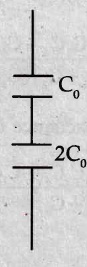
Parallel : \(C_{P}=C_{0}+C_{0}=2 C_{0}\)
Series : \(\frac{1}{C_{S}} =\frac{1}{C_{0}}+\frac{1}{2 C_{0}} \)
\(=\frac{2+1}{2 C_{0}} \)
\(\frac{1}{C_{S}} =\frac{3}{2} C_{0} \)
\(\therefore C_{s} =\frac{2}{3} C_{0} \)
Figure (b)
.jpg)
\(C_{p 1} =2 C_{0},C_{p 2} =2 C_{0}\)
\(\frac{1}{C_{S}} =\frac{1}{C_{p_{1}}}+\frac{1}{C_{P 2}}=\frac{1}{2 C_{0}}+\frac{1}{2 C_{0}} \)
\(\frac{1+1}{2 C_{0}} =\frac{2}{2 C_{0}}=\frac{1}{C_{0}} \)
\(\therefore C_{s} =C_{0} \)
Figure (c)
.jpg)
\(C_{p} =C_{0}+C_{0}=2 C_{0} \)
\(C_{p} =2 C_{0}+C_{0} \)
\(C_p=3 C_{0} \)
Figure (d)
.jpg)
\(\frac{1}{C_{s 1}}=\frac{1}{C_{1}}+\frac{1}{C_{2}}=\frac{C_{1}+C_{2}}{C_{1} C_{2}} \)
\(\therefore C_{S 1}=\frac{C_{1} C_{2}}{C_{1}+C_{2}} \) ....(1)
\(\frac{1}{C_{s 2}}=\frac{1}{C_{3}}+\frac{1}{C_{4}}=\frac{C_{4}+C_{3}}{C_{3} C_{4}} \)
\(\therefore C_{s 2}=\frac{C_{3} C_{4}}{C_{3}+C_{4}} \) ...(2)
\(C_{p} =C_{s 1}+C_{s 2} \)
\(C_p= \frac{C_{1} C_{2}}{C_{1}+C_{2}}+\frac{C_{3} C_{4}}{C_{3}+C_{4}} \)
\(=\frac{C_{1} C_{2}\left(C_{3}+C_{4}\right)+C_{3} C_{4}\left(C_{1}+C_{2}\right)}{\left(C_{1}+C_{2}\right)\left(C_{3}+C_{4}\right)} \)
\(C_{p} =\frac{\mathbf{C}_{1} C_{2} C_{3}+C_{1} C_{2} C_{4}+C_{3} \mathbf{C}_{4} C_{1}+C_{3} C_{4} C_{2}}{\left(C_{1}+C_{2}\right)\left(C_{3}+C_{4}\right)} \)
The Effective capacitance across PQ and RS is same.
\(C_{PQ}=C_{RS}=C=\frac{C_{1} C_{2} C_{3}+C_{2} C_{3} C_{4}+C_{1} C_{2} C_{4}+C_{1} C_{3} C_{4}}{\left(C_{1}+C_{2}\right)\left(C_{3}+C_{4}\right)}\)
Figure (e): Across PQ
.jpg)
\(\frac{1}{C_{S 1}}=\frac{1}{C_{0}}+\frac{1}{C_{0}}=\frac{2}{C_{0}} \)
\(\therefore C_{S 1}=\frac{C_{0}}{2} \)
\(\frac{1}{C_{S 2}}=\frac{1}{C_{0}}+\frac{1}{C_{0}}=\frac{2}{C_{0}} \)
\(C_{S 2}=\frac{C_{0}}{2} \)
\(C_{P}=C_{S 1}+C_{S 2}=\frac{C_{0}}{2}+\frac{C_{0}}{2} \)
\(C_p=C_{0} \)
Resultant Capacitance
.jpg)
CR = Co + Co
CR = 2Co
3.
Distance of separation d = 0.6 x 10⁻³ m
Electric field E = 3 x 10⁶ Vm-1
\(E=\frac{V}{d}\)
(a) Potential difference V = E x d
V = 3 x 106 x 0.6 x 10-3
V = 1800 V
(b) If the gap (distance d) is increased then potential difference would be increased, since V = E x d
(c) If E = 3 x 10⁶ Vm-1 and distance of separation d = 1 x 10⁻³ m
Potential difference V = E x d
V = 3 x 106 x 10-3
V = 3 x 103 = 3000 V
4.
(i) Electric field is given by \(|E|=\frac{d V}{d x}\)
(a) For region A,
dV = 8 - 5 = 3V, dx - (0.2 - 0) = 0.2m
\(\therefore E_{x}=\frac{d V}{d x}=\frac{3}{0.2}=15 \mathrm{Vm}^{-1}\)
(b) For region B,
dv = 0, Ex = 0
(c) For region C
dV = (7 - 5) = 2V, dx = (0.6 - 0.4) = 0.2 m
\(\therefore E_{x}=\frac{d V}{d x}=\frac{2}{0.2}=10 \mathrm{Vm}^{-1}\)
(d) For region D
dV = (7 - 1)=6V, dx = (0.8 - 0.6) = 0.2 m
\(\therefore E_{x}=\frac{d V}{d x}=\frac{6}{0.2}=30 \mathrm{Vm}^{-1}\)
(ii) Electric field as a function of x for Figure (ii).
5.
G = 6.67 x 10⁻¹¹ Nm2kg-2
Mass of Earth mE = 5.9 x 1024 kg
Mass of Moon mm = 7.9 x 10²² kg
Gravitational force \(F_{g}=\frac{G m_{E} \times m_{M}}{r^{2}}\); Electro static force \(F_e=k\frac{q \times q}{r^2}\)
By equating the forces, \( k\frac{q \times q}{r^{2}}=G \cdot \frac{m_{E} \times m_{M}}{r^{2}} \)
\(\because k=\frac{1}{4 \pi \varepsilon_{0}}=9 \times 10^{9} \)
\( 4 \pi \varepsilon_{0} =0.11 \times 10^{-9} \)
\(q =\sqrt{4 \pi \varepsilon_{0} G m_{E} \cdot m_{M}} \) ....(1)
\(=\sqrt{0.11 \times 10^{-9} \times 6.67 \times 10^{-11} \times 5.9 \times 10^{24} \times 7.9 \times 10^{22}}\)
\( q =\sqrt{34.2 \times 10^{26}} \)
q ≈ 5.85 x 10¹³ C
b) Suppose the distance (r) between Moon and Earth is halved, there is no change in the value of charge (q). Because from equation (1), q is independent of distance (r).
6.
From the figure F1 = F5 but opposite in direction. So cancel each other
Also, F2 sin 45o = F4 sin 45o but opposite in direction. So cancel each other.
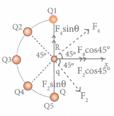
\( \mathrm{F}_{\mathrm{tot}} =\mathrm{F}_{3}+\mathrm{F}_{2} \cos 45^{\circ}+\mathrm{F}_{4} \cos 45^{\circ} \)
\(\mathrm{F}_{\mathrm{tot}} =\frac{k q Q}{R^{2}}+\frac{k q Q}{R^{2}} \frac{1}{\sqrt{2}}+\frac{k q Q}{R^{2}} \frac{1}{\sqrt{2}} \)
\(\mathrm{~F}_{\mathrm{tot}} =\frac{k q Q}{R^{2}}+2 \frac{k q Q}{R^{2}} \frac{1}{\sqrt{2}} \)
\(=\frac{k q Q}{R^{2}}+\sqrt{2} \sqrt{2} \frac{k q Q}{R^{2}} \frac{1}{\sqrt{2}} \)
\(\vec{F}_{\text {tot }} =\frac{k q Q}{R^{2}}[1+\sqrt{2}] \hat{i} N\)
\(\vec{F} =\frac{1}{4 \pi \varepsilon_{o}} \frac{q Q}{R^{2}}(1+\sqrt{2}) \hat{i N}\)
7.
(a) The electrostatic potential on the surface of the sphere A is VA = \(\frac { 1 }{ 4\pi { \epsilon }_{ 0 } } \frac { { q }_{ 1 } }{ { r }_{ 1 } } \)
The electrostatic potential on the surface of the sphere A is VB = \(\frac { 1 }{ 4\pi { \epsilon }_{ 0 } } \frac { { q }_{ 2 } }{ { r }_{ 2 } } \)
Since VA = VB. We have
\(\frac { { q }_{ 1 } }{ { r }_{ 1 } } =\frac { { q }_{ 2 } }{ { r }_{ 2 } } \Rightarrow { q }_{ 1 }=\left( \frac { { r }_{ 1 } }{ { r }_{ 2 } } \right) { q }_{ 2 }\)
But from the conservation of total charge, Q = q1 + q2, we get q1 = Q – q2. By substituting this in the above equation,
Q - q2 = \(\left( \frac { { r }_{ 1 } }{ { r }_{ 2 } } \right) { q }_{ 2 }\)
so that q2 = Q\(\left( \frac { { r }_{ 2 } }{ { r }_{ 1 }+{ r }_{ 2 } } \right) \)
Therefore,
q2 = 100 x 10-9 x \(\left( \frac { 2 }{ 10 } \right) \) = 20nC and q1 = Q - q2 = 80nC
The electric charge density for sphere A is σ1 = \(\frac { { q }_{ 1 } }{ 4\pi { r }_{ 1 }^{ 2 } } \)
The electric charge density for sphere B is σ2 = \(\frac { { q }_{ 2 } }{ 4\pi { r }_{ 2 }^{ 2 } } \)
Therefore,
σ1 = \(\frac { 80\times 10^{ -9 } }{ 4 \pi \times 64\times 10^{ -4 } } \) = 0.99 x 10⁻⁶ Cm-2 and
σ2 =\(\frac { 20\times 10^{ -9 } }{ 4\pi \times 4\times 10^{ -4 } } \) = 3.9 x 10⁻⁶ Cm-2
Note that the surface charge density is greater on the smaller sphere compared to the larger sphere (σ2 ≈ 4σ1) which confirms the result \(\frac { { \sigma }_{ 1 } }{ \sigma _{ 2 } } =\frac { { r }_{ 2 } }{ { r }_{ 1 } } \)
The potential on both spheres is the same. So we can calculate the potential on any one of the spheres
VA=\(\frac { 1 }{ 4\pi { \varepsilon }_{ 0 } } \frac { { q }_{ 1 } }{ { r }_{ 1 } } =\frac { 9\times 10^{ 9 }\times 80\times { 10 }^{ -9 } }{ 8\times 10^{ -2 } } \) = 9kV
8.
The capacitors 1 μF and 3μF are connected in parallel and 6μF and 2 μF are also separately connected in parallel. So these parallel combinations reduced to equivalent single capacitances in their respective positions, as shown in the figure (b).
Ceq = 1 + 3 = 4μF
Ceq = 6 + 2 = 8μF
From the figure (b), we infer that the two 4 μF capacitors are connected in series and the two 8 μF capacitors are connected in series. By using formula for the series, we can reduce to their equivalent capacitances as shown in figure (c).
\(\frac { 1 }{ { C }_{ eq } } =\frac { 1 }{ 4 } +\frac { 1 }{ 4 } =\frac { 1 }{ 2 } \) ⇒ Ceq = 2μF and
\(\frac { 1 }{ C_{ eq } } =\frac { 1 }{ 8 } +\frac { 1 }{ 8 } =\frac { 1 }{ 4 } \) ⇒ Ceq = 4μF
From the figure (c), we infer that 2μF and 4μF are connected in parallel. So the equivalent capacitance is given in the figure (d).
Ceq = 2 + 4 = 6μF
Thus the combination of capacitances in figure (a) can be replaced by a single capacitance 6 μF.
9.
(a) The capacitance of the capacitor in the presence of dielectric is
C = \(\frac { { \varepsilon }_{ r }{ \varepsilon }_{ 0 }A }{ d } =\frac { 5\times 8.85\times 10^{ -12 }\times 6 \times 10^{-4}}{ 6\times 10^{ -3 } } \)
= 44.25 x 10⁻¹³F = 4.425 pF
The stored charge is
Q = CV = 44.25 x 10-13 x 10
= 442.5 x 10⁻¹³C = 44.25pC
The stored energy is
\(U=\frac { 1 }{ 2 } \) CV2 = \(\frac { 1 }{ 2 } \) x 44.25 x 10-13 x 100
= 2.21 x 10⁻¹⁰ J
(b) After the removal of the dielectric, since the battery is already disconnected the total charge will not change. But the potential difference between the plates increases. As a result, the capacitance is decreased.
New capacitance is
C0=\(\frac { C }{ { \varepsilon }_{ r } } =\frac { 44.25\times 10^{ -12 } }{ 5 } \)
= 0.885 x 10⁻¹² F = 0.885 pF
The stored charge remains same and 44.25 pC. Hence newly stored energy is
U0 =\(\frac { { Q }^{ 2 } }{ 2{ C }_{ 0 } } =\frac { { Q }^{ 2 }{ \varepsilon }_{ r } }{ 2C } =\varepsilon _{ r }U\)
= 5 x 2.21 x 10-10J = 11.05 x 10⁻¹⁰J
The increased energy is ΔU = (11.05 - 2.21) x 10-10 J = 8.84 x 10⁻¹⁰ J
When the dielectric is removed, it experiences an inward pulling force due to the plates. To remove the dielectric, an external agency has to do work on the dielectric which is stored as additional energy. This is the source for the extra energy 8.84 x 10⁻¹⁰ J.
10.
11.
If the conductor has no net charge, then its motion is the same as usual projectile motion of a mass m which we studied in Kinematics (unit 2, vol-1 XI physics). Here, in this problem, in addition to downward gravitational force, the charge also will experience a downward uniform electrostatic force.
The acceleration of the charged ball due to gravity = -g\(\hat { j } \)
The acceleration of the charged ball due to uniform electric field =\(-\frac { qE }{ m } \hat { j } \)
The total acceleration of charged ball in downward direction \(\vec { a } =-\left( g+\frac { qE }{ m } \right) \vec { j } \)
It is important here to note that the acceleration depends on the mass of the object. Galileo’s conclusion that all objects fall at the same rate towards the Earth is true only in a uniform gravitational field. When a uniform electric field is included, the acceleration of a charged object depends on both mass and charge.
But still the acceleration a = \(\left( g+\frac { qE }{ m } \right) \) is constant throughout the motion. Hence we use kinematic equations to calculate the range, maximum height and time of flight. In fact we can simply replace g by \(g+\frac { qE }{ m } \) in the usual expressions of range, maximum height and time of flight of a projectile.
| Without charge | With the charge +q | |
| Time of flight T | \(\frac { 2v_{ 0 }sin\theta }{ g } \) | \(\frac { 2{ v }_{ 0 }sin\theta }{ \left( g+\frac { qE }{ m } \right) } \) |
| Maximum height hmax | \(\frac { { v }_{ 0 }^{ 2 }sin^{ 2 }\theta }{ 2g } \) | \(\frac { { v }_{ 0 }^{ 2 }sin^{ 2 }\theta }{ 2\left( g+\frac { qE }{ m } \right) } \) |
| Range R | \(\frac { { v }_{ 0 }^{ 2 }sin2\theta }{ g } \) | \(\frac { { v }_{ 0 }^{ 2 }sin2\theta }{ \left( g+\frac { qE }{ m } \right) } \) |
Note that the time of flight, maximum height, range are all inversely proportional to the acceleration of the object. Since \(\left( g+\frac { qE }{ m } \right) \) >g for charge +q, the quantities T, hmax, and R will decrease when compared to the motion of an object of mass m and zero net charge. Suppose the charge is –q, then \(\left( g-\frac { qE }{ m } \right) \)
12.
(a) Electric potential at point P is given by
Vp=\(\frac { 1 }{ 4\pi { \varepsilon }_{ 0 } } \frac { q }{ { r }_{ p } } =\frac { 9\times 10^{ 9 }\times 9\times { 10 }^{ -6 } }{ 10 } \) = 8.1 x 10³ V
Electric potential at point Q is given by
VQ = \(\frac { 1 }{ 4\pi { \varepsilon }_{ 0 } } \frac { q }{ { r }_{ Q } } =\frac { 9\times 10^{ 9 }\times 9\times { 10 }^{ -6 } }{ 16 } \) = 5.06 x 10³ V
Note that the electric potential at point Q is less than the electric potential at point P. If we put a positive charge at P, it moves from P to Q. However if we place a negative charge at P it will move towards the charge +9μC.
The potential difference between the points P and Q is given by
ΔV = Vp-VQ = +3.04 x 10³ V
b) Suppose we replace the charge +9 μC by -9 μC, then the corresponding potentials at the points P and Q are,
Vp = -8.1 x 10³ V, VQ = -5.06 x 10³ V
Note that in this case electric potential at the point Q is higher than at point P.
The potential difference or voltage between the points P and Q is given by
ΔV = Vp-VQ= -3.04 x 10³V
(c) The electric potential V at a point P due to some charge is defined as the work done by an external force to bring a unit positive charge from infinity to P. So to bring the q amount of charge from infinity to the point P, work done is given as follows.
W = qV
WQ = 2 x 10-6 x 5.06 x 103J = 10.12 x 10⁻³ J.
13.
Case (a)
The magnitude of the electric field at point P is
Ep = \(\frac { 1 }{ 4\pi \varepsilon _{ 0 } } \frac { q }{ { r }^{ 2 } } =\frac { 9\times { 10 }^{ 9 }\times 1\times 10^{ -6 } }{ 4 } \)
= 2.25 x 10³ NC-1
Since the source charge is positive, the electric field points away from the charge. So the electric field at the point P is given by
\(\bar { { E }_{ p } } \) = 2.25 x 10³ NC-1
For the point Q
\(|\vec { { E }_{ Q } } |=\frac { 9\times 10^{ 9 }\times 1\times { 10 }^{ -6 } }{ 16 } \) = 0.56 x 10³ NC-1
Hence \(\vec { { E }_{ Q } } \) = 0.56 x 10³\(\hat { j } \) NC-1
Case (b)
The magnitude of the electric field at point P
\(\bar { { E }_{ p } } =\frac { kq }{ r^{ 2 } } =\frac { 1 }{ 4\pi { \varepsilon }_{ 0 } } \frac { q }{ { r }^{ 2 } } =\frac { 9\times 10^{ 9 }\times 2\times 10^{ -6 } }{ 4 } \)
= 4.5 x 10³ NC-1
Since the source charge is negative, the electric field points towards the charge. So the electric field at the point P is given by
\(\vec { E_{ p } } \) = -4.5 x 10³\(\hat { i } \)NC-1
For the point Q, \(|\vec { { E }_{ Q } } |\frac { 9\times 10^{ 9 }\times 2\times { 10 }^{ -6 } }{ 36 } \)
= 0.5 x 10³ NC-1
\(\vec { E_{ Q } } \) = 0.5 x 10³\(\hat { i } \)NC-1
At the point Q the electric field is directed along the positive x-axis.
14.
According to the superposition principle, the total electrostatic force on charge q1 is the vector sum of the forces due to the other charges,
\(\vec { { F }_{ 1 }^{ tot } } =\bar { { F }_{ 12 } } +\bar { { F }_{ 13 } } +\bar { F_{ 14 } } \)
The following diagram shows the direction of each force on the charge q1.
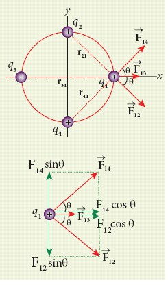
The charges q2 and q4 are equi-distant from q1. As a result the strengths (magnitude) of the forces \(\vec { { F }_{ 12 } } \) and \(\vec { { F }_{ 14 } } \) are the same even though their directions are different. Therefore the vectors representing these two forces are drawn with equal lengths. But the charge q3 is located farther compared to q2 and q4. Since the strength of the electrostatic force decreases as distance increases, the strength of the force \(\vec { { F }_{ 13 } } \) is lesser than that of forces \(\vec { { F }_{ 12 } } \) and \(\vec { { F }_{ 14 } } \). Hence the vector representing the force \(\vec { { F }_{ 13 } } \) is drawn with smaller length compared to that for forces \(\vec { { F }_{ 12 } } \) and \(\vec { { F }_{ 14 } } \).
From the figure, r21 =\(\sqrt { 2 } \) m = r41 and r31 = 2m
The magnitudes of the forces are given by
F13 = \(\frac { kq^{ 2 } }{ r_{ 31 }^{ 2 } } =\frac { 9\times 10^{ 9 }\times 10^{ -12 } }{ 4 } \)
F13 = 2.25 x 10⁻³ N
F12 = \(\frac { kq^{ 2 } }{ r_{ 31 }^{ 2 } } ={ F }_{ 14 }=\frac { 9\times 10^{ 9 }\times 10^{ -12 } }{ 2 } \)
= 4.5 x 10⁻³N
From the figure, the angle θ = 450. In terms of the components, we have
\(\vec { { F }_{ 12 } } ={ F }_{ 12 }cos\theta \hat { i } -{ F }_{ 12 }sin\theta \hat { j } \)
= 4.5 x 10⁻³ x \(\frac { 1 }{ \sqrt { 2 } } \hat { i-4.5\times { 10 }^{ -3 }\times \frac { 1 }{ \sqrt { 2 } } \hat { j } } \)
\(\vec { { F }_{ 13 } } =F_{ 13 }\hat { i } \) = 2.25 x 10⁻³ N\(\hat { i } \)
\(\vec { { F }_{ 14 } } ={ F }_{ 14 }cos\theta \hat { i } +{ F }_{ 14 }sin\theta \hat { j } \)
= 4.5 x 10⁻³ x \(\frac { 1 }{ \sqrt { 2 } } \hat { i+4.5\times { 10 }^{ -3 }\times \frac { 1 }{ \sqrt { 2 } } \hat { j } } \)
Then the total force on q1 is,
\(\vec { { F }_{ 1 }^{ tot } }={ (F }_{ 12 }cos\theta \hat { i } -{ F }_{ 12 }sin\theta \hat { j } )+{ F }_{ 13 }\hat { i } +{ (F }_{ 14 }cos\theta \hat { i } +{ F }_{ 14 }sin\theta \hat { j } )\)
\(\vec { { F }_{ 1 }^{ tot } } =({ F }_{ 12 }cos\theta +F_{13}+{ F }_{ 14 }cos\theta )\hat { i } +(-{ F }_{ 12 }sin\theta +{ F }_{ 14 }sin\theta )\)\(\hat { j } \)
Since F12 = F14, the j th component is zero.
Hence we have
\(\vec { { F }_{ 1 }^{ tot } } =({ F }_{ 12 }cos\theta +F_{13}+{ F }_{ 14 }cos\theta )\hat { i } \)
substituting the values in the above equation,
\(\left( \frac { 4.5 }{ \sqrt { 2 } } +2.25+\frac { 4.5 }{ \sqrt { 2 } } \right) \times10^{-3}\hat { i }=(4.5\sqrt { 2 } +2.25)\times 10^{-3}\hat { i } \)
\(\vec { { F }_{ 1 }^{ tot } } \) = 8.61 x 10⁻³ N\(\hat { i } \)
The resultant force is along the positive x-axis.
15.
The proton and the electron attract each other. The magnitude of the electrostatic force between these two particles is given by
\(F_e=\frac { ke^{ 2 } }{ { r }^{ 2 } } =\frac { 9\times 10^{ 9 }\times (1.6\times 10^{ -19 })^{ 2 } }{ (5.3\times 10^{ -11 })^{ 2 } } \)
=\(\frac { 9\times 2.56 }{ 28.09 } \) x 10-7 = 8.2 x 10⁻⁸ N
The gravitational force between the proton and the electron is attractive. The magnitude of the gravitational force between these particles is
FG = \(\frac { G{ m }_{ e }{ m }_{ p } }{ { r }^{ 2 } } \)
= \(\frac { 6.67\times 10^{ -11 }\times 9.1\times 10^{ -31 }\times 1.6\times 10^{ -27 } }{ (5.3\times 10^{ -11 })^{ 2 } } \)
= \(\frac { 97.11 }{ 28.09 } \) x 10-47 = 3.4 x 10-47N
The ratio of the two forces \(\frac { { F }_{ e } }{ F_{ G } } =\frac { 8.2\times 10^{ -8 } }{ 3.4\times 10^{ -47 } } \)
= 2.41 x 1039
Note that Fe ≈ 1039 FG
The electrostatic force between a proton and an electron is enormously greater than the gravitational force between them. Thus the gravitational force is negligible when compared with the electrostatic force in many situations such as for small size objects and in the atomic domain. This is the reason why a charged comb attracts an uncharged piece of paper with greater force even though the piece of paper is attracted downward by the Earth. This given figure is shown in below.
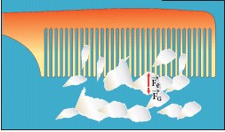
Electrostatic attraction between a comb and pieces of papers
16.
If the two spheres are neutral, the angle between them will be 0o when hanged vertically. Since they are positively charged spheres, there will be a repulsive force between them and they will be at equilibrium with each other at an angle of 30° with the vertical. At equilibrium, each charge experiences zero net force in each direction. We can draw a free-body diagram for one of the charged spheres and apply Newton’s second law for both vertical and horizontal directions.
The free-body diagram is shown below
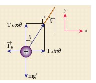
In the x-direction, the acceleration of the charged sphere is zero.
Using Newton’s second law \((\vec { { F }_{ tot }= } m\vec { a } )\), we have
T sinθ\(\hat { i } \) - Fe\(\hat { i } \) =0
T sinθ = Fe ......(1)
Here T is the tension acting on the charge due to the string and Fe is the electrostatic force between the two charges.
In the y-direction also, the net acceleration experienced by the charge is zero
Tcosθ\(\hat { j } \) - mg\(\hat { j } \) = 0
Tcosθ = mg ..(2)
By dividing equation (1) by equation (2),
tanθ = \(\frac { { F }_{ e } }{ mg } \) .....(3)
Since they are equally charged, the magnitude of the electrostatic force is
\({ F }_{ e }=k\frac { { q }^{ 2 } }{ { r }^{ 2 } } \) where k=\(\frac { 1 }{ 4\pi { \varepsilon }_{ 0 } } \)
Here r = 2a = 2Lsinθ. By substituting these values in equation (3),
tanθ = k\(\frac { { q }^{ 2 } }{ mg(2Lsin\theta )^{ 2 } } \) ..........(4)
Rearranging the equation (4) to get q
q = 2 Lsinθ\(\\ \sqrt { \frac { mgtan\theta }{ k } } \)
= 2 x 0.1 x sin 30o x \(\sqrt { \frac { 10^{ -3 }\times 10\times { tan30 }^{ 0 } }{ 9\times 10^{ 9 } } } \)
q = 8.01 x 10⁻⁸C = 80.1 nC
17.
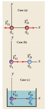
(a) q1 = +2 μC, q2 = +3 μC, and r = 1m. Both are positive charges. so the force will be repulsive.
Force experienced by the charge q2 due to q1 is given by
\(\vec { { F }_{ 21 } } =\frac { 1 }{ 4\pi { \varepsilon }_{ 0 } } \frac { { q }_{ 1 }{ q }_{ 2 } }{ { r }^{ 2 } } \hat { r_{ 12 } } \)
Here \(\hat { r_{ 12 } } \) is the unit vector from q1 to q2. Since q2 is located on the right of q1, we have
\(\hat { r_{ 12 } } =\hat { i } \), and \(\frac { 1 }{ 4\pi { \varepsilon }_{ 0 } }=9 \times10^9\) so that
\(\vec { { F }_{ 21 } } =\frac { 9\times 10^{ 9 }\times 2\times 10^{ -6 }\times 3\times 10^{ -6 } }{ 1^{ 2 } } \hat { i } \)
= 54 x 10-3 N\(\hat { i } \)
According to Newton’s third law, the force experienced by the charge q1 due to q2 is \(\vec { { F }_{ 12 } } =-\vec { { F }_{ 21 } } \) Therefore,
\(\vec { F_{ 12 } } \)= 54 x 10-3 N\(\hat { i } \)
The directions of \(\vec { { F }_{ 21 } } \) and \(\vec { { F }_{ 12 } } \) are shown in the figure (case (b)).
(b) q1 = +2 μC, q2 = –3 μC, and r = 1m. They are unlike charges. So the force will be attractive.
Force experienced by the charge q2 due to q1 is given by
\( \vec{F}_{21} =\frac{9 \times 10^{9} \times\left(2 \times 10^{-6}\right) \times\left(-3 \times 10^{-6}\right)}{1^{2}} \hat{r}_{12} \)
\(=-54 \times 10^{-3} \mathrm{~N} \hat{i}\left(\mathrm{Using} \hat{r}_{12}=\hat{i}\right)\)
The charge q2 will experience an attractive force towards q1 which is in the negative x direction.
According to Newton’s third law, the force experienced by the charge q1 due to q2 is \(\vec{F}_{12}=-\vec{F}_{21}\) Therefore,
\(\vec{F}_{12}=54 \times 10^{-3} \widehat{i} \mathrm{~N}\)
The directions of \(\vec{F}_{21} \text { and } \vec{F}_{12}\) are shown in the figure (case (b)).
(c) If these two charges are kept inside the water, then the force experienced by q2 due to q1
\(\vec { { F }_{ 21 }^{ W } } =\frac { 1 }{ 4\pi { \varepsilon }_{ 0 } } \frac { { q }_{ 1 }{ q }_{ 2 } }{ { r }^{ 2 } } \hat { r_{ 12 } } \)
since ε = εrε0,
we have \(\vec { { F }_{ 21 }^{ W } } =\frac { 1 }{ 4\pi { { \varepsilon }_{ r }\varepsilon }_{ 0 } } \frac { { q }_{ 1 }{ q }_{ 2 } }{ { r }^{ 2 } } \hat { r_{ 12 } } =\frac { \vec { F_{ 21 } } }{ { \varepsilon }_{ r } } \)
Therefore,
\(\vec { { F }_{ 21 }^{ W } } =\frac { 54\times { 10 }^{ -3 }N }{ 80 } \hat { i } \) = -0.675 x 10⁻³ N\(\hat { i } \)
18.

12th Standard Syllabus & Materials
12th Standard
TN 12th Computer Applications களப்பெயர் முறைமை (DNS) Sample Question Papers Study Material - QB365 Set A
NEW12th Standard
TN 12th Computer Applications வலையமைப்பு எடுத்துக்காட்டுகள் மற்றும் நெறிமுறைகள் Sample Question Papers Study Material - QB365 Set A
NEW12th Standard
TN 12th Computer Applications கணினி வலையமைப்பு ஓர் அறிமுகம் Sample Question Papers Study Material - QB365 Set A
NEW12th Standard
TN 12th Computer Applications PHP-உடன் MySQL-ஐ இணைத்தல் Sample Question Papers Study Material - QB365 Set A



Tamilnadu Stateboard 12th Standard Subjects

Maths

Chemistry
Physics

Biology

Computer Science

Business Maths and Statistics

Economics

Commerce

Accountancy

History

Computer Applications
Biology
Computer Technology
Computer Applications
Computer Science
Business Maths and Statistics
Commerce
Economics
Maths
Chemistry
Physics
Computer Technology
History
Accountancy

Tamil

English

French
Tamilnadu Stateboard Standards

