
 100% FREE ACCESS
12th Standard Syllabus & Materials
12th Standard
TN 12th Computer Applications மின்னணு தரவு பரிமாற்றம் Sample Question Papers Study Material - QB365 Set A
NEW12th Standard
TN 12th Computer Applications மின் - வணிக பாதுகாப்பு அமைப்புகள் Sample Question Papers Study Material - QB365 Set A
NEW12th Standard
TN 12th Computer Applications மின்னணு செலுத்தல் முறைகள் Sample Question Papers Study Material - QB365 Set A
NEW12th Standard
TN 12th Computer Applications மின் - வணிகம் Sample Question Papers Study Material - QB365 Set A
NEW12th Standard
TN 12th Computer Applications திறந்த மூல கருத்துருக்கள் Sample Question Papers Study Material - QB365 Set A
NEW12th Standard
TN 12th Computer Applications வலையமைப்பு வடமிடல் Sample Question Papers Study Material - QB365 Set A

Published on: 01/09/2022
QB365 provides a detailed and simple solution for every Possible Book Back Questions in Class 12 Physics Subject - Electrostatics, English Medium. It will help Students to get more practice questions, Students can Practice these question papers in addition to score best marks.
Download Tamil Nadu 12th Standard Physics question papers, model tests, one-mark questions, important questions, and public exam papers in PDF format. Free study materials and answer keys for TN State Board students.
Questions + Answers key
Take MCQ Physics Test1.
Explain in detail the construction and working of a Van de Graaff generator.
2.
Explain in detail how charges are distributed in a conductor, and the principle behind the lightning conductor.
3.
Derive the expression for resultant capacitance, when capacitors are connected in series and in parallel.
4.
Explain in detail the effect of a dielectric placed in a parallel plate capacitor.
5.
Explain dielectrics in detail and how an electric field is induced inside a dielectric.
6.
Explain the process of electrostatic induction.
7.
Discuss the various properties of conductors in electrostatic equilibrium.
8.
Obtain the expression for electric field due to an uniformly charged spherical shell.
9.
Obtain the expression for electric field due to an charged infinite plane sheet.
10.
11.
Derive an expression for electrostatic potential due to an electric dipole.
12.
Calculate the electric field due to a dipole on its axial line and equatorial plane.
13.
Consider a point charge +q placed at the origin and another point charge -2q placed at a distance of 9 m from the charge +q. Determine the point between the two charges at which electric potential is zero.
14.
Obtain the expression for energy stored in the parallel plate capacitor.
15.
Obtain the expression for capacitance for a parallel plate capacitor.
16.
Obtain Gauss law from Coulomb’s law.
17.
Derive an expression for electrostatic potential energy of the dipole in a uniform electric field.
18.
Obtain an expression for potential energy due to a collection of three point charges which are separated by finite distances.
19.
Derive an expression for electrostatic potential due to a point charge.
20.
Derive an expression for the torque experienced by a dipole due to a uniform electric field.
21.
Define ‘Electric field’ and discuss its various aspects.
22.
Explain in detail Coulomb’s law and its various aspects.
23.
Discuss the basic properties of electric charges.
1.
In the year 1929, Robert Van de Graaff designed a machine which produces a large amount of electrostatic potential difference, up to several million volts (107 V).
Principle:
Electrostatic induction and Action at points.
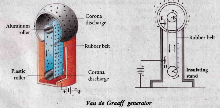
Construction:
(i) A large hollow spherical conductor is fixed on the insulating stand as shown in Figure. A pulley B is mounted at the center of the hollow sphere and another pulley C is fixed at the bottom. A belt made up of insulating materials like silk or rubber runs over both pulleys. The pulley C is driven continuously by the electric motor. Two comb-shaped metallic conductors E and D are fixed near the pulleys.
(ii) The comb D is maintained at a positive potential of 104 V by a power supply. The upper comb E is connected to the inner side of the hollow metal sphere
Working:
(i) Because of the high electric field near comb D, air between the belt and comb D gets ionized. The positive charges are pushed towards the belt and negative charges are attracted towards the comb D.
(ii) The positive charges stick to the belt and move up. When the positive charges reach the comb E, a large amount of negative and positive charges are induced on either side of comb E due to electrostatic induction.
(iii) As a result, the positive charges are pushed away from the comb E and they reach the outer surface of the sphere. Since the sphere is a conductor, the positive charges are distributed uniformly. on the outer surface of the hollow sphere.
(iv) At the same time the negative charges nullify the positive Charges in the belt due to corona discharge before it passes over the pulley.
(v) When the belt descends, it has almost no net charge. At the bottom, it again gains a large positive charge. The belt goes up and delivers the positive charges to the outer surface of the sphere.
(vi) This process continues until the outer surface produces the potential difference of the order of 107 which is the limiting value. We cannot store charges beyond this limit since the extra charge starts leaking to the surroundings due to ionization of air. The leakage of charges can be reduced by enclosing the machine in a gas filled steel chamber at very high pressure.
(vii) The high voltage produced in this Van de Graaff generator is used to accelerate positive ions (protons and deuterons) for nuclear disintegrations and other applications.
2.
Distribution of charges in a conductor:
(i) Consider two conducting spheres A and B of radii r1 and r2 respectively connected to each other by a thin conducting wire as shown in the Figure. The distance between the spheres is much greater than the radii of either spheres.
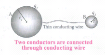
(ii) If a charge Q is introduced into any one of the spheres, this charge Q is redistributed into both the spheres such that the electrostatic potential is same in both the spheres. They are now uniformly charged and attain electrostatic equilibrium. Let q1 be the charge residing on the surface of sphere A and q2 is the charge residing on the surface of sphere B such that Q = q1 + q2, The charges are distributed only on the surface and there is no net charge inside the conductor.
The electrostatic potential at the surface of the sphere A is given by
\({ V }_{ A }=\frac { 1 }{ 4\pi { \varepsilon }_{ 0 } } \frac { { q }_{ 1 } }{ { r }_{ 1} } \quad \quad ...(1)\)
(iii) The electrostatic potential at the surface of the sphere B is given by ,
\({ V }_{ B }=\frac { 1 }{ 4\pi { \varepsilon }_{ 0 } } \frac { { q }_{ 2 } }{ { r }_{ 2 } } \) ...(2)
iv) The surface of the conductor is an equipotential. Since the spheres are connected by the conducting wire, the surfaces of both the spheres together form an equipotential surface.
This implies that
VA= VB
or \(\frac { { q }_{ 1 } }{ { r }_{ 1 } } =\frac { { q }_{ 2 } }{ { r }_{ 2 } } \) ...(3)
v) Let us take the charge density on the surface of sphere A and charge density on the surface of sphere B is σ2.This implies that q1 = 4πr12σ1 and 4πr22σ2 substituting these values into equation (3), we get
σ1r1 = σ2r2 ...(4)
from which we conclude that σr = constant ...(5)
Lightning conductor:
It is used to protect tall buildings from lightning strikes.
Principle:
(i) Action at points (or) corona discharge.
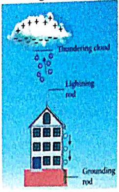
(ii) This device consists of a long thick copper rod passing from top of the building to the ground.
(iii) The upper end of the rod has a sharp spike or a sharp needle as shown in Figure.
(iv) The lower end of the rod is connected to copper plate which is buried deep into the ground.
(v) When a negatively charged cloud is passing above the building, it causes a positive charge on the spike. Since the induced charge density on thin sharp spike is large, it results in a corona discharge. This positive Charge ionizes the surrounding air which in turn neutralizes the negative charge in the cloud.
(vi) The negative charge pushed to the spikes passes through the copper rod and is safely diverted to the Earth. The lightning arrester does not stop the lightning; rather it diverts the lightning to the ground safely.
3.
(a) Capacitor in series
(i) Consider three capacitors of capacitance C1, C2 and C3 connected in series with a battery of voltage V as shown in the Figure (a).
(ii) As soon as the battery is connected to the capacitors in series, the electrons of charge -Q are transferred from negative terminal to the right plate of C3 which pushes the electrons of same amount -Q from left plate of C3 to the right plate of C2 due to electrostatic induction.
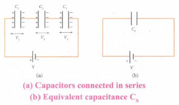
(iii) Similarly, the left plate of C2 pushes the charges of -Q to the right plate of C1 which induces the positive charge +Q on the left plate of C1.
(iv) At the same time, electrons of charge -Q are transferred from left plate of C1 to positive terminal of the battery.
(v) By these processes, each capacitor stores the same amount of charge Q.
(vi) The capacitances of the capacitors are in general different so that the voltage across each capacitor is also different and are denoted as V1, V2 and V3 respectively.
(vii) The sum voltage across capacitor must be equal to the voltage of the battery.
V = V1 + V2 + V3 ....(1)
Since, Q = CV
We have V = \(\frac { Q }{ { C }_{ 1 } } +\frac { Q }{ { C }_{ 2 } } +\frac { Q }{ { C }_{ 3 } } \)
\(=Q\left[ \frac { 1 }{ { C }_{ 1 } } +\frac { 1 }{ { C }_{ 2 } } +\frac { 1 }{ { C }_{ 3 } } \right] ...(2)\)
(viii) If three capacitors in series are considered to form an equivalent single capacitor Cs shown in Figure (b), then we have \(V=\frac { Q }{ { C }_{ s } } \). Substituting this expression into equation (2), we get
\(\frac { Q }{ { C }_{ s } } =Q\left( \frac { 1 }{ { C }_{ 1 } } +\frac { 1 }{ { C }_{ 2 } } +\frac { 1 }{ { C }_{ 3 } } \right) \)
\(\frac { 1 }{ { C }_{ s } } =\frac { 1 }{ { C }_{ 1 } } +\frac { 1 }{ { C }_{ 2 } } +\frac { 1 }{ { C }_{ 3 } } \) ...(3)
(ix) Thus, the inverse of the equivalent capacitance Cs of three capacitors connected in series is equal to the sum of the inverses of each capacitance. This equivalent capacitance Cs, is always less than the smallest individual capacitance in the series.
(b) Capacitor in parallel
i) Consider three capacitors of capacitance C1, C2 and C3 connected in parallel with a battery of voltage V as shown in Figure (a).
ii) Since corresponding sides of the capacitors are connected to the same positive and negative terminals of the battery, the voltage across each capacitor is equal to the battery's voltage.
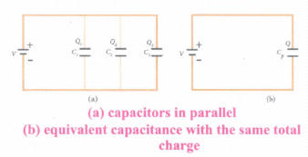
iii) Since capacitance of the capacitors is different, the charge stored in each capacitor is not the same. Let the charge stored in the three capacitors be Q1, Q2, and Q3 respectively.
iv) According to the law of conservation of total charge, the sum of these three charges is equal to the charge Q transferred by the battery,
Q = Q1 + Q2 + Q3 ...(4)
Now, since Q = CV, we have
Q = C1V + C2V + C3V ...(5)
(v) If these three capacitors are considered to form a single capacitance C, which stores the total charge Q as shown in the Figure (b), then we can write Q = CpV. Substituting this in equation (2), we get
CpV = C1V + C2V + C3V
Cp = C1+ C2 + C3 ...(6)
vi) Thus, the equivalent capacitance of capacitors connected in parallel is equal to the sum of the individual capacitances.
vii) The equivalent capacitance Cp, in a parallel connection is always greater than the largest individual capacitance. In a parallel connection, it is equivalent as area of each capacitance adds to give more effective area such that total capacitance increases.
4.
Effect of dielectrics in capacitors:
Suppose dielectrics like mica, glass or paper are introduced between the plates, then the capacitance of the capacitor is altered. The dielectric can be inserted into the plates in two different ways.
(i) when the capacitor is disconnected from the battery.
(ii) when the capacitor is connected to the battery.
(i) When the capacitor is disconnected from the battery
Consider a capacitor with two parallel plates each of cross-sectional area A and are separated by a distance d. The capacitor is charged by a battery of voltage Vo and the charge stored is Qo. The capacitance of the capacitor without the dielectric is,
\(C_{0}=\frac{Q_{0}}{V_{0}}\) ....(i)
The battery is then disconnected from the capacitor and the dielectric is inserted between the plates. This is shown in Figure.
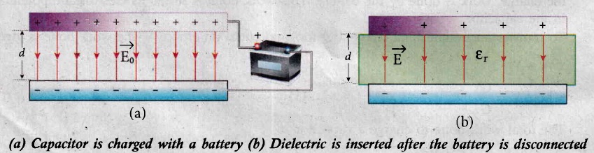
The introduction of dielectric between the plates will decrease the electric field. Experimentally it is found that the modified electric field is given by,
\(E=\frac{E_{0}}{\varepsilon_{r}}\) ....(2)
Here Eo is the electric field inside the capacitors when there is no dielectric and \(\varepsilon_{\mathrm{r}}\) is the relative permittivity of the dielectric or simply known as the dielectric constant. Since \(\varepsilon_{\mathrm{r}}\) > 1, the electric field E < Eo.
As a result, the electrostatic potential difference between the plates (V = Ed) is also reduced. But at the same time, the charge Qo will remain constant once the battery is disconnected.
Hence the new potential difference is
\(V=E d=\frac{E_{0}}{\varepsilon_{r}} d=\frac{V_{0}}{\varepsilon_{r}}\) .......(3)
We know that capacitance is inversely proportional to the potential difference. Therefore as V decreases, C increases.
Thus new capacitance in the presence of a dielectric is
\(C=\frac{Q_{0}}{V}=\varepsilon_{r} \frac{Q_{0}}{V_{0}}=\varepsilon_{r} C_{0}\) ......(4)
Since \(\varepsilon_{\mathrm{r}}\) > 1, we have C > Co. Thus insertion of the dielectric increases the capacitance.
We know that, Co =\(\frac{\varepsilon_{\mathrm{o}} A}{d}\) ...........(5)
Equation (4) ⇒ \(C=\frac{\varepsilon_{r} \varepsilon_{0} A}{d}=\frac{\varepsilon A}{d} \) ..........(6)
where \(\varepsilon=\varepsilon_{\mathrm{r}} \varepsilon_{\mathrm{o}}\) is the permittivity of the dielectric medium.
The energy stored in the capacitor before the insertion of a dielectric is given by,
\(U_{0}=\frac{1}{2} \frac{Q_{0}^{2}}{C_{0}}\) .......(7)
After the dielectric is inserted, the charge Qo remains constant but the capacitance is increased. As a result, the stored energy is decreased.
\(U=\frac{1}{2} \frac{Q_{0}^{2}}{C}=\frac{1}{2} \frac{Q_{0}^{2}}{\varepsilon_{r} C_{0}}=\frac{U_{0}}{\varepsilon_{r}}\) ..........(8)
Since \(\varepsilon_{\mathrm{r}}\) > 1we get U < Uo. There is a decrease in energy because, when the dielectric is inserted, the capacitor spends some energy in pulling the dielectric inside.
(ii) When the battery remains connected to the capacitor:
When the battery of voltage vo remains connected to the capacitor and the dielectric is inserted into the capacitor, then
(a) The potential difference vo across the plates remains constant.
(b) The charge stored in the capacitor is increased by a factor \(\varepsilon_{\mathrm{r}}\). (Experimentally found).
.jpg)
\({Q}=\varepsilon_{r} Q_{0}\) .......(1)
Due to this increased charge, the capacitance is also increased. The new capacitance is,
\(C=\frac{Q}{V_{0}}=\varepsilon_{r} \frac{Q_{0}}{V_{0}}=\varepsilon_{r} C_{0}\) ......(2)
However the reason for the increase in capacitance in this case where the battery remains connected is different from the case when the battery is disconnected before introducing the dielectric.
The energy stored in the capacitor before the insertion of a dielectric is given by,
\(U_{0}=\frac{1}{2} C_{0} V_{0}^{2}\) ....(4)
After the dielectric is inserted, the capacitance is increased; hence the stored energy is also increased.
\( U=\frac{1}{2} C V_{0}^{2}=\frac{1}{2} \varepsilon_{r} C_{0} V_{0}^{2}=\varepsilon_{r} U_{0} \) .....(5)
\(Since \ \varepsilon_{r}>1\ we \ have \ U>U_{o}.\)
Note: Here we have not used the expression \(U_o=\frac{1}{2}\frac{Q_0^2}{C_0}\)because here, both charge and capacitance are changed, whereas in equation (4), Vo remains constant.
Since voltage between the capacitor Vo is constant, the electric field between the plates also remains constant .The energy density is given by,
\(u=\frac{1}{2} \varepsilon E_{0}^{2}\) ..(6)
where ε is the permittivity of the given dielectric material.
5.
Dielectrics or insulators:
(a) A dielectric is a non-conducting material and has no free electrons. The electrons in a dielectric are bound within the atoms Example : Ebonite, glass and mica are some examples of dielectrics.
(b) A dielectric is made up of either polar molecules or non-polar molecules.
Non-polar molecules:
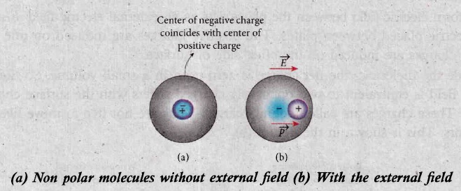
(a) A non-polar molecule is one in which centers of positive and negative charges coincide. As a result, it has no permanent dipole moment. Examples of non-polar molecules are hydrogen (H2), oxygen (O2) and carbon dioxide (CO2) etc.
(b) When an external electric field is applied, the centres of positive and negative charges are separated by a small distance which induces dipole moment in the direction of the external electric field. Then the dielectric is said to be polarized by an external electric field. This is shown in Figure.
Polar molecules
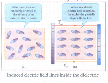
(a) In polar molecules, the centres of the positive and negative charges are separated even in the absence of an external electric field. They have a permanent dipole moment. Due to thermal motion, the direction of each dipole moment is oriented randomly (Figure (a)). Hence the net dipole moment is zero in the absence of an external electric field. Examples of polar molecules are H2O, N2O, HCl, NH3.
(b) When an external electric field is applied, the dipoles inside the polar molecule tend to align in the direction of the electric field. Hence a net dipole moment is induced in it. Then the dielectric is said to be polarized by an external electric field (Figure (b).
.jpg)
Polarisation:
(a) In the presence of an external electric field, the dipole moment is induced in the dielectric material. Polarisation P is defined as the total dipole moment per unit volume of the dielectric. For most dielectrics (linear isotropic), the Polarisation is directly proportional to the strength of the external electric field. This is written as
\(\vec{P}=\chi_{e} \vec{E}_{e x t}\) .....(2)
where \(\chi_{e}\) is a constant called the electric susceptibility which is a characteristic of each dielectric.
Induced Electric Field inside the dielectric:
(i) When an external electric field is applied on a conductor, the charges are aligned in such a way that an internal electric field is created which cancels the external electric field. But in the case of a dielectric, which has no free electrons, the external electric field only realigns the charges so that an internal electric field is produced.
(ii) The magnitude of the internal electric field is smaller than that of external electric field. Therefore the net electric field inside the dielectric is not zero but is parallel to an external electric field with magnitude less than that of the external electric field.
For example let us consider a rectangular dielectric slab placed between two oppositely charged plates (capacitor) as shown in the Figure (c).
(iii) The uniform electric field between the plates acts as an external electric field \(\vec { E } \)ext which polarizes the dielectric placed between plates. The positive charges are induced on one side surface and negative charges are induced on the other side of surface.
(iv) But inside the dielectric, the net charge is zero even in a small volume. So the dielectric in the external field is equivalent to two oppositely charged sheets with the surface charge densities +σb and -σb. These charges are called bound charges. They are not free to move like free electrons in conductors. This is shown in the Figure (c).
(v) For example, the charged balloon after rubbing sticks onto a wall. The reason is that the negatively charged balloon is brought near the wall, it polarizes induces opposite charges on the surface of the wall, which attracts the balloon.
6.
Electrostatic induction:
(i) Let us Consider an uncharged (neutral) conducting sphere at rest on an insulating stand. Suppose a negatively charged rod is brought near the conductor without touching it, as shown in Figure (a).
The negative charge of the rod repels the electrons in the conductor to the opposite side. As a result, positive charges are induced near the region of the charged rod while negative charges on the farther side.
Before introducing the charged rod, the free electrons were distributed uniformly on the surface of the conductor and the net charge is zero. Once the charged rod is brought near the conductor, the distribution is no longer uniform with more electrons located on the farther side of the rod and positive charges are located closer to the rod. But the total charge is zero.
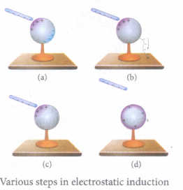
(ii) Now the conducting sphere is connected to the ground through a conducting wire. This is called grounding. Since the ground can always receive any amount of electrons, grounding removes the electron from the conducting sphere. Note that positive charges will not flow to the ground because they are attracted by the negative charges of the rod Figure (b).
(iii) When the grounding wire is removed from the conductor, the positive charges remain near the charged rod Figure (c).
(iv) Now the charged rod is taken away from the conductor. As soon as the charged rod is removed, the positive charge gets distributed uniformly on the surface of the conductor Figure (d). By this process, the neutral conducting sphere becomes positively charged.
7.
A conductor at electrostatic equilibrium has the following properties:
(i) The electric field is zero everywhere inside the conductor. This is true regardless of whether the conductor is solid or hollow:
(a) This is an experimental fact. Suppose the electric field is not zero inside the metal, then there will be a force on the mobile charge carriers due to this electric field.
(b) As a result, there will be a net motion of the mobile charges, which contradicts the conductors being in electrostatic equilibrium. Thus the electric field is zero everywhere inside the conductor. We can also understand this fact by applying an external uniform electric field on the conductor.
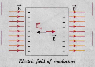
(c) Before applying the external electric field, the free electrons in the conductor are uniformly distributed in the conductor. When an electric field is applied, the free electrons accelerate to the left causing the left plate to be negatively charged and the right plate to be positively charged as shown in Figure.
(d) Due to this realignment of free electrons, there will be an internal electric field created inside the conductor which increases until it nullifies the external electric field.
(e) Once the external electric field is nullified the conductor is said to be in electrostatic equilibrium. The time taken by a conductor to reach electrostatic equilibrium is in the order of 10-16 s, which can be taken as almost instantaneous.
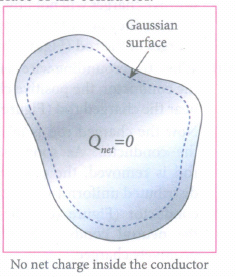
(ii) There is no net charge inside the conductors. The charges must reside only on the surface of the conductors:
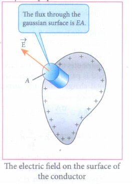
(a) We can prove this property using Gauss law. Consider an arbitrarily shaped conductor as shown in Figure. A Gaussian surface is drawn the conductor such that it is very close to the surface of the conductor.
(b) Since the electric field is zero everywhere inside the conductor, the net electric flux is also zero over this Gaussian surface. From Gauss's law, this implies that there is no net charge inside the conductor.
(c) Even if some charge is introduced inside the conductor, it immediately reaches the surface of the conductor.
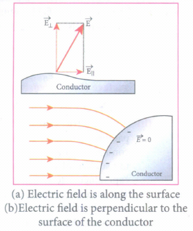
(iii) The electric field outside the conductor is perpendicular to the surface of the conductor and has a magnitude of \(\frac { \sigma }{ { \varepsilon }_{ 0 } } \) is the surface charge density at that point:
(a) If the electric field has components parallel to the surface of the conductor, then free electrons on the surface of the conductor would experience acceleration (Figure a).
(b) This means that the conductor is not in equilibrium. Therefore at electrostatic equilibrium, the electric field must be perpendicular to the surface of the conductor. This is shown in Figure (b).
(c) We now prove that the electric field has magnitude \(\frac { \sigma }{ { \varepsilon }_{ 0 } } \) just outside the conductor's surface.
(d) Consider a small cylindrical Gaussian surface, as shown in the Figure. One-half of this cylinder is embedded inside the conductor.
(e) Since electric field is normal to the surface of the conductor, the curved part of the cylinder has zero electric flux.
(f) Also inside the conductor, the electric field is zero. Hence the bottom flat part of the Gaussian surface has no electric flux.
(g) Therefore the top flat surface alone contributes to the electric flux. The electric field is parallel to the area vector and the total charge inside the surface is σA. By applying Gaus's law,
\(EA=\frac { \sigma A }{ { \varepsilon }_{ 0 } } \)
In vector form, \(\vec { E } =\frac { \sigma }{ { \varepsilon }_{ 0 } } \hat { n } \) ....(1)
(h) Where \(\hat { n } \) represents the unit vector outward normal to the surface of the conductor. Suppose \(\sigma\) < 0, then electric field points inward perpendicular to the surface.
(iv) The electrostatic potential has the same value on the surface and inside of the conductor :
(a) We know that the conductor has no parallel electric component on the surface which means that charges can be moved on the surface without doing any work.
(b) This is possible only if the electrostatic potential is constant at all points on the surface and there is no potential difference between any two points on the surface.
(c) Since the electric field is zero inside the conductor, the potential is the same as the surface of the conductor. Thus at electrostatic equilibrium, the conductor is always at equipotential.
8.
Electric field due to a uniformly charged spherical shell :
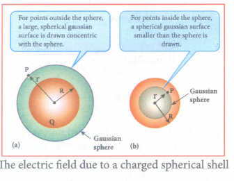
Consider a uniformly charged spherical shell of radius R carrying total charge Q as shown in Figure. The electric field at points outside and inside the sphere is found using Gauss law.
Case (a): At a point outside the shell (r > R):
(i) Let us choose a point P outside the shell at a distance r from the centre.
(ii) The charge is uniformly distributed on the surface of the sphere (spherical symmetry).
(iii) Hence the electric field must point radially outward if Q > 0 and point radially inward if Q < 0. So, a spherical Gaussian surface of radius r is chosen and the total charge enclosed by this Gaussian surface is Q. Applying Gauss law,
\(\oint _{ Gaussian\ surface }^{ }{ \vec { E } .d\vec { A } } =\frac { Q_{encl} }{ { \varepsilon }_{ 0 } } \quad \quad \quad ....(1)\)
(iv) The electric field \(\vec { E } \) and \(d\vec { A } \) point in the same direction (outward normal) at all the points on the Gaussian surface. The magnitude of \(\vec { E } \) is also the same at all points due to the spherical symmetry of the charge distribution.
\( E\oint _{ Gaussian\ surface }^{ }{ dA=\frac { Q }{ { \varepsilon }_{ 0 } } ....(2) } \)
But \(\oint _{ Curved\ surface }^{ }{ dA } \) = total area of Gaussian surface = \(4\pi { r }^{ 2 }\).
Substituting this in equation (2),
\(E.4\pi { r }^{ 2 }=\frac { Q }{ { \varepsilon }_{ 0 } } \)
\(E.4\pi { r }^{ 2 }=\frac { Q }{ { \varepsilon }_{ 0 } } (or)\quad E=\frac { 1 }{ 4\pi { \varepsilon }_{ 0 } } \frac { Q }{ { r }^{ 2 } } \)
In vector form \(\vec { E } =\frac { 1 }{ 4\pi { \varepsilon }_{ 0 } } \frac { Q }{ { r }^{ 2 } } \hat { r } \quad ....(3)\)
(v) The electric field is radially outward if Q > 0 and radially inward if Q < O. From equation (3), the electric field at a point outside the shell will be same as if the entire charge Q is concentrated at the center of the spherical shell.
Case (b): At a point on the surface of the spherical shell (r = R):
The electrical field at points on the spherical shell (r = R) is given by
\(\vec { E } =\frac { Q }{ 4\pi { \varepsilon }_{ 0 }{ R }^{ 2 } } \hat { r } \quad \quad \quad ...(4)\).
Case (c): At a point inside the spherical shell (r < R):
(vi) Consider a point P inside the shell at a distance r from the centre. A Gaussian sphere of radius r is constructed as shown in the figure. Applying Gauss law,
\(\oint _{ Gaussian\ surface }^{ }{ \vec { E } .d\vec { A } } =\frac { Q }{ \varepsilon_0 } \)
\(E.4\pi r^2 =\frac { Q }{ \varepsilon_0 } \) .....(5)
(vii) Since Gaussian surface encloses no charge, Q = 0. The cquation (5) becomes
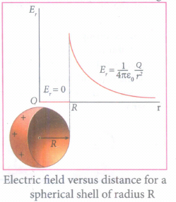
E = 0 (r < R) .....(6)
(viii) The electric field due to the uniformly charged spherical shell is zero at all points inside the shell. A graph is plotted between the electric field and radial distaance.
9.
Electric field due to charged infinite plane sheet:
(i) Consider an infinite plane sheet of charges with uniform surface charge density σ. (Charge per unit area). Let P be a point at a distance of r from the sheet as shown in the Figure.
(ii) Since the plane is infinitely large, the electric field should be same at all points equidistant from the plane and radially directed outward at all points. A cylindrical-shaped Gaussian surface of length 2r and two flat surfaces is chosen such that the infinite plane sheet passes perpendicularly through the middle part of the Gaussian surface.
Total electric flux linked with the cylindrical surface,
\({ \phi }_{ E }=\int { \vec { E } .d\vec { A } } \)
\(=\int _{ Curved\ surface }^{ }{ \vec { E } .d\vec { A } } +\int _{ P }^{ }{ \vec { E } .d\vec { A } + } \int _{ P^{'} }^{ }{ \vec { E } .d\vec { A } } =\frac { { Q }_{ encl } }{ { \varepsilon }_{ 0 } } \quad ...(1)\)
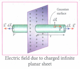
(iii) The electric field is perpendicular to the area element at all points on the curved surface and is parallel to the surface areas at P and P ' (Figure). Then, applying Gauss's law.
\({ \phi }_{ E }=\int _{ p }^{ }{ EdA+ } \int _{ p' }^{ }{ EdA= } \frac { { Q }_{ encl } }{ { \varepsilon }_{ 0 } } \quad ...(2)\)
Since the magnitude of the electric field at these two equal flat surfaces is uniform, E is taken out of the integration and Qncel is given by Qencl = σA, we get
\(2E\int _{ p }^{ }{ dA=\frac { \sigma A }{ { \varepsilon }_{ 0 } } } \)
The total area of surface either at P or P'
\(\int _{ p }^{ }{ dA=A } \)
Hence \(2EA=\frac { \sigma A }{ { \varepsilon }_{ 0 } }\) or \(E=\frac { \sigma }{ 2{ \varepsilon }_{ 0 } } \quad \quad \quad \quad ...(3)\)
In vector \(\vec { E } =\frac { \sigma }{ 2{ \varepsilon }_{ 0 } } \hat { n } \quad \quad \quad \quad ...(4)\)
(iv) Here \(\hat { n } \) is the outward unit vector normal to the plane. Note that the electric field due to an infinite plane sheet of charge depends on the surface charge density and is independent of the distance r.
(v) The electric field will be the same at any point farther away from the charged plane.
(vi) Equation (4) implies that if σ > 0 the electric field at any point P is outward perpendicular \(\hat { n } \) to the plane and if σ < 0 the electric field points inward perpendicularly (\(-\hat { n } \)) to the plane.
10.
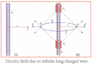
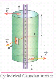
11.
Electrostatic potential at a point due to an electric dipole :
(i) Consider two equal and opposite charges separated by a small distance 2a as shown in Figure. The point P is located at a distance r from the midpoint 'O' of the dipole. Let θ be the angle between the line OP and dipole axis AB.

(ii) Let r1 be the distance of point P from +q and r2 be the distance of point P from -q.
Potential at P due to charge +q\(=\frac { 1 }{ 4\pi { \varepsilon }_{ 0 } } \frac { q }{ { r }_{ 1 } } \)
Potential at P due to charge -q \(=-\frac { 1 }{ 4\pi { \varepsilon }_{ 0 } } \frac { q }{ { r }_{ 2 } } \)
Total potential at the point P,
\(V=\frac { 1 }{ 4\pi { \varepsilon }_{ 0 } } q\left( \frac { 1 }{ { r }_{ 1 } } -\frac { 1 }{ { r }_{ 2 } } \right) \) ....(1)
(iii) Suppose if the point P is far away from the dipole, such that (r >> a), then equation (1) can be expressed in terms of r.
By the cosine law for triangle BOP,
\({ r }_{ 1 }^{ 2 }={ r }^{ 2 }+{ a }^{ 2 }-2ra cos\theta \)
\({ r }_{ 1 }^{ 2 }={ r }^{ 2 }\left( 1+\frac { { a }^{ 2 } }{ { r }^{ 2 } } -\frac { 2a }{ r } cos\theta \right) \)
Since the point P is very far from dipole, then(r >> a). Then term \(\frac{a^{2}}{r^{2}}\)
\({ r }_{ 1 }^{ 2 }={ r }^{ 2 }\left( 1-2a\frac { cos\theta }{ r } \right) \)
\((or){ r }_{ 1 }=r{ \left( 1-\frac { 2a }{ r } cos\theta \right) }^{ \frac { 1 }{ 2 } }\)
\(\frac { 1 }{ { r }_{ 1 } } =\frac { 1 }{ r } { \left( 1-\frac { 2a }{ r } cos\theta \right) }^{ -\frac { 1 }{ 2 } }\)
iv) Since \(\frac{a}{r}\) << 1, we can use binomial theorem and retain the terms up to first order.
\(\frac { 1 }{ { r }_{ 1 } } =\frac { 1 }{ r } \left( 1+\frac { a }{ r } cos\theta \right) ...(2)\)
Similarly applying the cosine law for triangle AOP,
r22 = r2 + a2 - 2ra cos (180-θ)
Since cos(180 - θ) = - cos θ we get
r22= r2 + a2 + 2ra cos θ
Neglecting the term \(\frac { { a }^{ 2 } }{ { r }^{ 2 } } \) because (r >> a)
\({ r }_{ 2 }^{ 2 }={ r }^{ 2 }\left( 1+\frac { 2acos\theta }{ r } \right) \)
\({ r }_{ 2 }=r{ \left( 1+\frac { 2acos\theta }{ r } \right) }^{ \frac { 1 }{ 2 } }\)
Using Binomial theorem, we get
\(\frac { 1 }{ { r }_{ 2 } } =\frac { 1 }{ r } \left( 1-a\frac { cos\theta }{ r } \right) \quad \quad ...(3)\)
Substituting equation (3) and (2) in equation (1),
\(V=\frac { 1 }{ 4\pi { \varepsilon }_{ 0 } } q\left( \frac { 1 }{ r } \left( 1+a\frac { cos\theta }{ r } \right) -\frac { 1 }{ r } \left( 1-a\frac { cos\theta }{ r } \right) \right) \)
\(V=\frac { q }{ 4\pi { \varepsilon }_{ 0 } } \left( \frac { 1 }{ r } \left( 1+a\frac { cos\theta }{ r } -1+a\frac { cos\theta }{ r } \right) \right) \)
\(V=\frac { 1 }{ 4\pi { \varepsilon }_{ 0 } } \frac { 2aq }{ { r }^{ 2 } } cos\theta \)
v)
\(V=\frac { 1 }{ 4\pi { \varepsilon }_{ 0 } } \left( \frac { pcos\theta }{ { r }^{ 2 } } \right) \)
Now we can write p cos\(\theta =\vec { p } .\hat { r } \) where \(\hat { r } \) is the unit vector from the point O to point P. Hence the electric potential at a point P due to an electric dipole is given by
\(V=\frac { 1 }{ 4\pi { \varepsilon }_{ 0 } } \frac { \vec { p } .\hat { r } }{ { r }^{ 2 } } (r>>a)\quad ...(4)\)
Equation (4) is valid for distances very large compared to the size of the dipole. But for a point dipole, the equation (4) is valid for any distance.
Special cases:
Case (i) : If the point P lies on the axial line of the dipole on the side of +q, then θ = 0. Then the electric potential becomes
\(V=\frac { 1 }{ 4\pi { \varepsilon }_{ 0 } } \frac { p }{ { r }^{ 2 } } \quad \quad ...(5)\)
Case (ii) : If the point P lies on the axial line of the dipole on the side of -q, then θ = 180°, then
\(V=-\frac { 1 }{ 4\pi { \varepsilon }_{ 0 } } \frac { p }{ { r }^{ 2 } } \quad \quad ...(6)\)
Case (iii) : If the point P lies on the equatorial line of the dipole, then θ = 90°. Hence,
V = 0 .....(7)
12.
Case (i): Electric field due to an electric dipole at points on the axial Iine:
Consider an electric dipole placed on the x-axis as shown in Figure. A point C is located at a distance of r from the midpoint O (of the dipole) along the axial line.
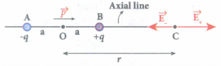
The electric field at a point C due to +q is
\({ \vec { E } }_{ + }=\frac { 1 }{ 4\pi { \varepsilon }_{ 0 } } \frac { q }{ { (r-a) }^{ 2 } } \) along BC
Since the electric dipole moment vector \(\vec { p } \) is from -q to +q and is directed along BC, the above equation is rewritten as
\({ \vec { E } }_{ + }=\frac { 1 }{ 4\pi { \varepsilon }_{ 0 } } \frac { q }{ { (r-a) }^{ 2 } } \hat { p } \) ....(1)
When \(\vec { p } \) is the electric dipole moment unit vector from -q to +q. The electric field at a point C due to -q is
\({ \vec { E } }_{ - }=-\frac { 1 }{ 4\pi { \varepsilon }_{ 0 } } \frac { q }{ { (r+a) }^{ 2 } } \hat { p } \) ....(2)
Since +q is located closer to the point C than -q, \({ \vec { E } }_{ + }\) is stronger than \({ \vec { E } }_{ - }\). Therefore, the length of the \({ \vec { E } }_{ + }\) vector is drawn larger than that of \({ \vec { E } }_{ - }\) vector.
The total electric field at point C is calculated using the superposition principle of the electric field.
\({ \vec { E } }_{ tot }={ \vec { E } }_{ + }+{ \vec { E } }_{ - }\)
\(=\frac { 1 }{ 4\pi { \varepsilon }_{ 0 } } \frac { q }{ { (r-a) }^{ 2 } } \hat { p } -\frac { 1 }{ 4\pi { \varepsilon }_{ 0 } } \frac { q }{ { (r+a) }^{ 2 } } \hat { p } \)
\({ \vec { E } }_{ tot }=\frac { q }{ 4\pi { \varepsilon }_{ 0 } } \left( \frac { 1 }{ { (r-a) }^{ 2 } } -\frac { 1 }{ { (r+a) }^{ 2 } } \right) \hat { p } \) ....(3)
\({ \vec { E } }_{ tot }=\frac { 1 }{ 4\pi { \varepsilon }_{ 0 } } q\left( \frac { 4ra }{( { r }^{ 2 }-{ a }^{ 2 })^2 } \right) \hat { p } \) ...(4)
Note that the total electric field is along \({ \vec { E } }_{ + }\), since +q is closer to C than -q.
If the point C is very far away from the dipole then (r >> a). Under this limit the term \(({ r }^{ 2 }-{ a }^{ 2 })\approx { r }^{ 2 }\).
Substituting this into equation (4), we get
\({ \vec { E } }_{ tot }=\frac { 1 }{ 4\pi { \varepsilon }_{ 0 } } \left( \frac { 4aq }{ { r }^{ 3 } } \right) \hat { p } (r>>a)\)
\(since\quad 2aq\hat { p } =\vec { p } \)
\({ \vec { E } }_{ tot }=\frac { 1 }{ 4\pi { \varepsilon }_{ 0 } } \frac { 2\vec { p } }{ { r }^{ 3 } } (r>>a)\) ...(5)
The direction \({ \vec { E } }_{ tot }\) is shown in Figure.
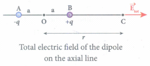
NOTE: If the point C is chosen on the left side of the dipole, the total electric field is still in the direction of \(\vec { p } \).
Case (ii) Electic field due to an electric dipole at a point on the equatorial plane:
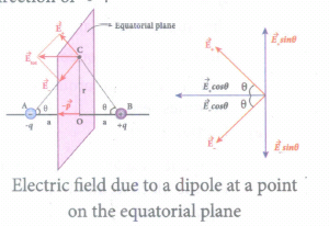
Consider a point C at a distance r from the midpoint O of the dipole on the equatorial plane. Since the point C is equidistant from +q and -q, the magnitude of the electric fields of +q and -q are the same. The direction of \({ \vec { E } }_{ + }\) is along BC and the direction of \({ \vec { E } }_{ - }\) is along CA. \({ \vec { E } }_{ + }\) and \({ \vec { E } }_{ - }\) are resolved into two components; one component parallel to the dipole axis and the other perpendicular to it. The perpendicular components \(|{ \vec { E } }_{ + }|\) sinθ and \(|{ \vec { E } }_{ -}|\) sinθ are equal in magnitude and oppositely directed and cancel each other. The magnitude of the total electric field at point C is the sum of the parallel components of \({ \vec { E } }_{ + }\) and \({ \vec { E } }_{ - }\) and its direction is along \(-\hat{p}\) as shown in the Figure.
\({ \vec { E } }_{ tot }=-|{ \vec { E } }_{ + }|cos\theta \hat { p } -|{ \vec { E } }_{ - }|cos\theta \hat { p } \) ...(6)
The magnitudes \({ \vec { E } }_{ + }\) and \({ \vec { E } }_{ - }\) are the same and given by,
\(|{ \vec { E } }_{ + }|=|{ \vec { E } }_{ - }|=\frac { 1 }{ 4\pi { \varepsilon }_{ 0 } } \frac { q }{ (r^2+a^2) } \) ...(7)
By substituting equation (7) into equation (6), we get
\({ \vec { E } }_{ tot }=\frac { 1 }{ 4\pi { \varepsilon }_{ 0 } } \frac { 2qcos\theta }{ ({ r }^{ 2 }+{ a }^{ 2 }) } \hat { p } ....(8)\)
\(=-\frac { 1 }{ 4\pi { \varepsilon }_{ 0 } } \frac { 2qa }{ ({ r }^{ 2 }+{ a }^{ 2 })^{ \frac { 3 }{ 2 } } } \hat { p } \)
Since \(cos \theta =\frac { a }{ \sqrt { { r }^{ 2 }+{ a }^{ 2 } } } \)
\({ \vec { E } }_{ tot }=\frac { 1 }{ 4\pi { \varepsilon }_{ 0 } } \frac { \vec { p } }{ ({ r }^{ 2 }+{ a }^{ 2 })^{ \frac { 3 }{ 2 } } } \)
Since \(\vec { p } \) = 2qa\(\hat { p } \) ...(9)
At very large distances (r >> a), the equation (9) becomes
\({ \vec { E } }_{ tot }=\frac { 1 }{ 4\pi { \varepsilon }_{ 0 } } \frac { \vec { p } }{ { r }^{ 3 } } (r>>a)\) ...(10)
Negative sign shows that direction of Electric field is opposite to the direction of dipole moment vector.
13.
According to the superposition principle, the total electric potential at a point is equal to the sum of the potentials due to each charge at that point.
Consider the point at which the total potential zero is located at a distance x from the charge +q as shown in the figure.
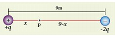
The total electric potential at P is zero.
Vtot = \(\frac { 1 }{ 4\pi { \varepsilon }_{ 0 } } \left( \frac { q }{ x } -\frac { 2q }{ (9-x) } \right) \)=0
Which gives \(\frac { q }{ x } -\frac { 2q }{ (9-x) } \)
or \(\frac { 1 }{ x } =\frac { 2 }{ (9-x) } \)
Hence, x = 3m
14.
Energy stored in the capacitor
i) Capacitor not only stores the charge but also it stores energy. When a battery is connected to the capacitor, electrons of total charge - Q are transferred from one plate to the other plate. To transfer the charge, work is done by the battery. This work done is stored as electrostatic potential energy in the capacitor.
ii) To transfer an infinitesimal charge dQ for a potential difference V, the work done is given by
dW = V dQ
Where \(V=\frac { Q }{ C } \) .....(1)
iii) The total work done to charge a capacitor is
\(W=\int _{ 0 }^{ Q }{ \frac { Q }{ C } } dQ=\frac { { Q }^{ 2 } }{ 2C } \quad \quad ....(2)\)
This work done is stored as electrostatic potential energy (UE) in the capacitor.
\({ U }_{ E }=\frac { { Q }^{ 2 } }{ 2C } =\frac { 1 }{ 2 } { CV }^{ 2 },\quad (\therefore Q=CV)\quad ....(3)\)
(iv) This stored energy is thus directly proportional to the capacitance of the capacitor and the square of the voltage between the plates of the capacitor.Substituting \(C=\frac { { \varepsilon }_{ 0 }A }{ d } \) and V = Ed.
\(U=\frac { 1 }{ 2 } \left( \frac { { \varepsilon }_{ 0 }A }{ d } \right) { (Ed) }^{ 2 }=\frac { 1 }{ 2 } { \varepsilon }_{ 0 }(Ad){ E }^{ 2 }\quad \quad \quad \quad \quad ...(4)\)
where Ad = volume of the space between the capacitor plates. The energy stored per unit volume of space is defined as energy density \({ u }_{ E }=\frac { U }{ Volume } \)
Equation (4) ⇒ \({ u }_{ E }=\frac{1}{2}{ \varepsilon }_{ 0 }{ E }^{ 2 }\).....(5)
(v) From equation (5),
(a) We infer that the energy is stored in the electric field existing between the plates of the capacitor. Once the capacitor is allowed to discharge, the energy is retrieved.
(b) The energy density depends only on the electric field and not on the size of the plates of the capacitor.
(c) This is true for the electric field due to any type of charge configuration.
15.
Capacitance of a parallel plate capacitor:
(i) Consider a capacitor with two parallel plates each of cross-sectional area A and separated by a distance d as shown in Figure.
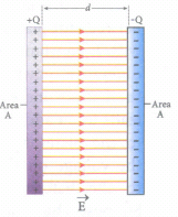
(ii) The electric field between two infinite parallel plates is uniform and is given by \(E=\frac { \sigma }{ { \varepsilon }_{ o} } \) where σ is the surface charge density on the plates \(\left( \sigma =\frac { Q }{ A } \right) \).
iii) If the separation distance d is very much smaller than the size of the plate (d2 < < A), then the above result is used even for finite-sized parallel plate capacitor.
The electric field between the plates is
\(E=\frac { Q }{ A{ \varepsilon }_{ 0 } } ...(1)\)
iv) Since the electric field is uniform, the electric potential between the plates having separation d is given by
\(V=Ed=\frac { Qd }{ A{ \varepsilon }_{ 0 } } \quad \quad \quad ...(2)\)
Therefore the capacitance of the capacitor is given by
\(C=\frac { Q }{ V } =\frac { Q }{ \left( \frac { Qd }{ A{ \varepsilon }_{ 0 } } \right) } =\frac { { \varepsilon }_{ 0 }A }{ d } \quad \quad ....(3)\)
(v) From equation (3), it is evident that capacitance is directly proportional to the area of cross section and is inversely proportional to the distance between the plates.
16.
Gauss law:
(i) A positive point charge Q is surrounded by an imaginary sphere of radius r as shown in Figure. then the total electric flux through the closed surface of the sphere is
\(\Phi_E =\oint { \vec { E } .d\vec { A } =\oint { Ed } Acos\theta } \) .....(1)
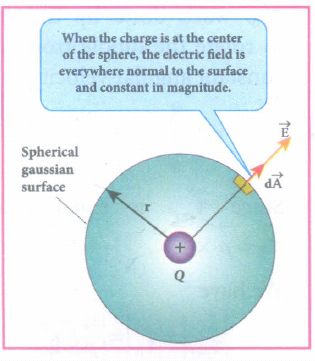
(ii) The electric field of the point charge is directed radially outward at all points on the surface of the sphere. Therefore, the direction of the area element \(d\vec { A } \) is along the electric field \(\vec { E } \) and θ = 0o.
\(\\ \Phi_E =\oint { EdA } \) Since cos0o = 1 ......(2)
iii) E is uniform on the surface of the sphere,
\(\\ \Phi_E=E\oint { dA } \) .......(3)
Substituting for \(\oint { dA=4{ \pi r }^{ 2 } } \) and \(E=\frac { 1 }{ 4\pi { \varepsilon }_{ 0 } } \frac { Q }{ { r }^{ 2 } } \) in eqn (3), we get
\(\therefore \phi E=4{ \pi r }^{ 2 }E\)
\({ \phi }_{ E }=\frac { 1 }{ 4\pi { \varepsilon }_{ 0 } } \frac { Q }{ { r }^{ 2 } } \times { 4\pi r }^{ 2 }=4\pi \frac { 1 }{ 4\pi { \varepsilon }_{ 0 } } Q\)
\({ \phi }_{ E }=\frac { Q }{ { \varepsilon }_{ 0 } } \) .....(4)
The equation (4) is called as Gauss's law.
17.
(i) Consider a dipole placed in the uniform electric field \(\vec { E } \). A dipole experiences a torque when kept in an uniform electric field \(\vec { E } \).(ii) To rotate the dipole (at constant angular velocity) from its initial angle θ' to another angle θ against the torque exerted by the electric field, an equal and opposite external torque must be applied on the dipole.
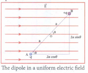
(iii) The work done by the external torque to rotate the dipole from angle θ' to θ at constant angular velocity is
\(W=\int _{ \theta ' }^{ \theta }{ { \tau }_{ ext }d\theta } \quad ...(1)\)
(iv) Since \({ \vec { \tau } }_{ ext }\) is equal and opposite to \({ \vec { \tau } }_{ E }=\vec { p } \times \vec { E } \), We have
\(|{ \vec { \tau } }_{ ext }|={ |\vec { \tau } }_{ E }|=|\vec { p } \times \vec { E } |\quad \quad \quad ...(2)\)
Substituting equation (2) in equation (1), we get
\(W=\int _{ \theta ' }^{ \theta }{ pEsin\theta d\theta } \)
\(W=pE(cos\theta '-cos\theta )\)
(v) This work done is equal to the potential energy difference between the angular positions θ to θ'.
U(θ) - U(θ') = ∆U= - pE cosθ + pE cosθ'
If the initial angle is θ' = 90o and is take as reference point, then U(θ') = pE cos 90o = 0. The potential energy stored in the system of dipole kept in the uniform electric field is given by
\(U=-pEcos\theta =-\vec { p } .\vec { E } \) ....(3)
In addition to p and E, the potential energy also depends on the orientation θ of the electric dipole with respect to the external electric field.
(vi) The potential energy is a) maximum when the dipole is aligned anti-parallel (θ = π) to the external electric field
b) minimum when the dipole is aligned parallel (θ = 0) to the external electric field.
18.
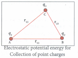
To calculate the total electrostatic potential energy, we use the following procedure. We bring all the charges one by one and arrange them according to the configuration as shown in Figure.
a) Bringing a charge q1 from infinity to the point A requires no work, because there are no other charges already present in the vicinity of charge q1.
b) To bring the second charge q2 to the point B, work must be done against the electric field created by the charge q1. So the work done on the charge q2 is W = q2 V1B. Here V1B is the electrostatic potential due to the charge q1 at point B.
\(U_I=\frac{1}{4\piε_o}\frac{q_1q_2}{r_{12}}\) .....(1)
Note that the expression is same when q2 is brought first and then q1 later.
c) Similarly to bring the charge q3 to the point C, work has to be done against the total electric field due to both the charges q1 and q2. So the work done to bring the charge q3 = q3 (V1C + V2C). Here V1C is the electrostatic potential due to charge q1 at point C and V2C is the electrostatic potential due to charge q2 at point C.
The electrostatic potential is
\(U_{II}=\frac{1}{4\piε_o}(\frac{q_1q_2}{r_{13}}+\frac{q_2q_3}{r_{23}})\) .....(2)
d) Adding equations (1) and (3), the total electrostatic potential energy for the system of three charges q1, q2 and q3 is
U = UI + UII
\(U=\frac{1}{4\piε_o}(\frac{q_1q_2}{r_{12}}+\frac{q_2q_3}{r_{13}}+\frac{q_2q_3}{r_{23}})\) ....(3)
19.
Electric potential due to a point charge:
Consider a positive charge q kept fixed at the origin. Let P be a point at distance r from the charge q. This is shown in Figure.
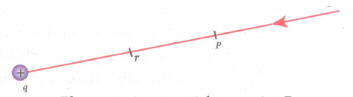
Electrostatic potential at a point P
The electric potential at the point P is
\(V=\int _{ \infty }^{ r }{ \left( -\vec { E } \right) d\vec { r } } =-\int _{ \infty }^{ r }{ \vec { E } } .d\vec { r } \) ...(1)
Electric field due to positive point charge q is
\(\vec { E } =\frac { 1 }{ 4\pi { \varepsilon }_{ 0 } } \frac { q }{ { r }^{ 2 } } \hat { r } \)
\(V=\frac { -1 }{ 4\pi { \varepsilon }_{ 0 } } \int _{ \infty }^{ r }{ \frac { q }{ { r }^{ 2 } } \hat { r } .d\vec { r } } \)
The infinitesimal displacement vector, \(d\vec { r } =dr\hat { r } \) and using \(\hat { r } \).\(\hat { r } \) = 1, we have
\(V=\frac { 1 }{ 4\pi { \varepsilon }_{ 0 } } \int _{ \infty }^{ r }{ \frac { q }{ { r }^{ 2 } } \hat { r } .dr\hat { r } =\frac { 1 }{ 4\pi { \varepsilon }_{ 0 } } \int _{ \infty }^{ r }{ \frac { q }{ { r }^{ 2 } } dr } } \)
After the integration,
\(V=-\frac { 1 }{ 4\pi { \varepsilon }_{ 0 } } q{ \left\{ -\frac { 1 }{ r } \right\} }_{ \infty }^{ r }=\frac { 1 }{ 4\pi { \varepsilon }_{ 0 } } \frac { q }{ r } \)
Hence, the electric potential due to a point charge q at a distance r is
\(V=\frac { 1 }{ 4\pi { \varepsilon }_{ 0 } } \frac { q }{ r } \) ....(2)
20.
Torque experienced by an electric dipole in the uniform electric field:
Consider an electric dipole of dipole moment \(\vec { p } \) placed in a uniform electric field \(\vec { E } \) whose field lines are equally spaced and point in the same direction. The charge +q will experience a force \(q\vec { E } \) in the direction of the field and charge -q will experience a force \(-q\vec { E } \) in a direction opposite to the field. Since the external field \(\vec { E } \) is uniform, the total force acting on the dipole is zero. These two forces acting at different points will constitute a couple and the dipole experience a torque. This torque tends to rotate the dipole.
The total torque on the dipole about the point O
\(\vec{\tau}=\overrightarrow{O A} \times(-q \vec{E})+\overrightarrow{O B} \times q \vec{E}\) ......(1)
Using right-hand corkscrew rule, it is found that total torque is perpendicular to the plane of the paper and is directed into it.
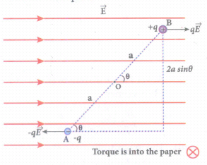
The magnitude of the total torque
\(\tau =|\vec { OA } |\left( -q\vec { E } \right) |sin\theta +|\vec { OB } ||\vec { E } |sin\theta \)
\(\tau =qE.2a\quad sin\theta \) ....(2)
where θ is the angle made by \(\vec { p } \) with \(\vec { E } \) since p = 2aq, the torque is written in terms of the vector product as
\(\vec { \tau } =\vec { p } \times \vec { E } \) ...(3)
The magnitude of this torque is \(\tau \) = pEsin \(\theta \) and is maximum when θ = 90o.
This torque tends to rotate the dipole and align it with the electric field \(\vec{E}\). Once \(\vec{p}\) is aligned with \(\vec{E}\), the total torque on the dipole becomes zero.
21.
The electric field at the point P at a distance r from the point charge q is defined as the force that would be experienced by a unit positive charge placed at that point and is given by,
\(\vec{E}=\frac{\vec{F}}{q_{0}}=\frac{k q}{r^{2}} \hat{r}=\frac{1}{4 \pi \varepsilon_{0}} \frac{q}{r^{2}} \hat{r}\) ....(1)
where \(\hat{r}\) is the unit vector pointing from q to the point of interest P.
Important aspect of the Electric field:
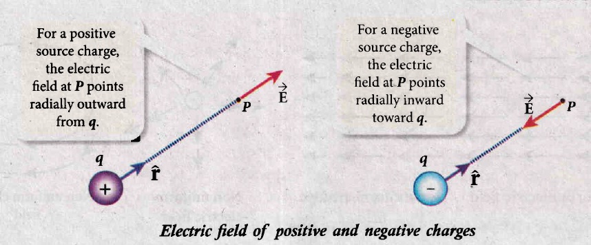
(i) If the charge q is positive then the electric field points away from the source charge and if q is negative, the electric field points towards the source charge q. This is shown in the Figure
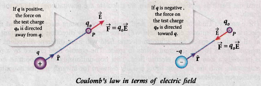
(ii) If the electric field at a point P is \(\vec{E},\) then the force experienced by the test charge qo placed at the point P is \(\vec { F } ={ q }_{ 0 }\vec { E } \)
This is Coulomb's law in terms of electric field. This is shown in Figure
(iii) The equation (1) implies that the electric field is independent of the test charge qo and it depends only on the source charge q.
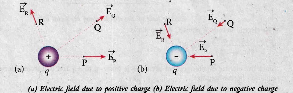
(iv) Since the electric field is a vector quantity, at every point in space, this field has unique direction and magnitude, as shown in Figures (a) and (b). From equation (1), we can infer that as distance increases, the electric field decreases in magnitude. Note that in Figures (a) and (b) the length of the electric field vector is shown for three different points. The strength or magnitude of the electric field at point P is stronger than at the points Q and R because the point P is closer to the source charge.
(v) In the definition of electric field, it is assumed that the test charge (q0) is taken sufficiently small, so that bringing this test charge will not move the source charge. In other words, the test charge is made sufficiently small such that it will not modify the electric field of the source charge.
(vi) The expression (1) is valid only for point charges. For continuous and finite size charge distributions, integration techniques must be used. These will be explained later in the same section. However, this expression can be used as an approximation for a finite-sized charge if the test point is very far away from the finite sized source charge. Note that we similarly treat the Earth as a point mass when we calculate the gravitational field of the Sun on the Earth.
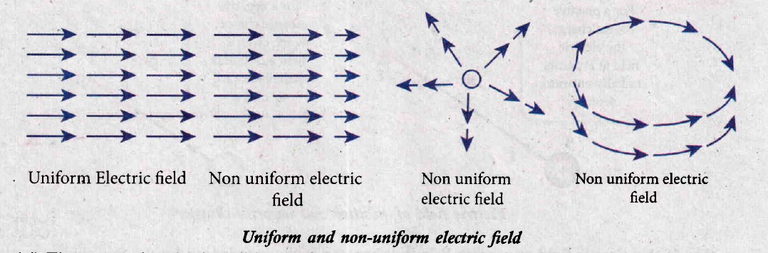
(vii) There are two kinds of the electric field : uniform or constant electric field and non-uniform electric field. Uniform electric field will have the same direction and constant magnitude at all points in space. Non-uniform electric field will have different directions or different magnitudes or both at different points in space. The electric field created by a point charge is basically a non uniform electric field. This non-uniformity arises, both in direction and magnitude, with the direction being radially outward (or inward) and the magnitude changes as distance increases. These are shown in Figure.
22.
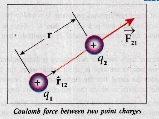
(i) Consider two point charges q1 and q2 at rest in vacuum, and separated by a distance of r, as shown in the figure.
(ii) According to Coulomb, the force on the point charge q2 exerted by another point charge q1 is \(\overrightarrow{F_{21}}=k \frac{q_{1} q_{2}}{r^{2}} \hat{r}_{12}\)
(iii) where \(\hat{r}_{12}\) is the unit vector directed from charge q1 to charge q2 and k is the proportionality constant.
Important aspects of Coulomb’s law
(i) Coulomb’s law states that the electrostatic force is directly proportional to the product of the magnitude of the two point charges and is inversely proportional to the square of the distance between the two point charges.
(ii) The force on the charge q2 exerted by the charge q1 always lies along the line joining the two charges. \({ \hat { r } }_{ 12 }\) is the unit vector pointing from charge q1 to q2. It is shown in the Figure. Likewise, the force on the charge q1 exerted by q2 is along \(-{ \hat { r } }_{ 12 }\)(i.e., in the direction opposite to \({ \hat { r } }_{ 12 })\).
(iii) In SI units, \(k=\frac { 1 }{ 4\pi { \varepsilon }_{ 0 } } \) and its value is k = 9 x 10⁹ Nm2C-2. Here \({ \varepsilon }_{ 0 }\) is the permittivity of free space or vacuum and the value of \({ \varepsilon }_{ 0 }=\frac { 1 }{ 4\pi k } =8.85\times { 10 }^{ -12 }{ C }^{ 2 }{ N }^{ -1 }{ m }^{ -2 }\).
(iv) The magnitude of the electrostatic force between two charges each of one coulomb and separated by a distance of 1 m is calculated as follows: \(|F|=\frac { 9\times { 10 }^{ 9 }\times 1\times 1 }{ { 1 }^{ 2 } } =9\times { 10 }^{ 9 }N\).
(v) In SI units, Coulomb's law in vacuum takes the form \({ \vec { F } }_{ 21 }=\frac { 1 }{ { 4\pi \varepsilon }_{ 0 } } \frac { { q }_{ 1 }{ q }_{ 2 } }{ { r }^{ 2 } } { \hat { r } }_{ 12 }.\) In a medium of permittivity \(\varepsilon \), the force between two point charges is given by\({ \vec { F } }_{ 21 }=\frac { 1 }{ 4\pi \varepsilon } \frac { { q }_{ 1 }{ q }_{ 2 } }{ { r }^{ 2 } } { \hat { r } }_{ 12 }\). Since \(\varepsilon \)>\(\varepsilon \)0, the force between two point charges in a medium other than vacuum is always less than that in vacuum. The relative permittivity for a given medium as \({ \varepsilon }_{ r }=\frac { \varepsilon }{ { \varepsilon }_{ 0 } } \) For vacuum or air, \(\varepsilon \)r = 1 and for all other media \(\varepsilon \)r > 1.
(vi) (a) Coulomb's law has same structure as Newton's law of gravitation. Both are inversely proportional to the square of the distance between the particles.
(b) The electrostatic force is directly proportional to the product of the magnitude of two point charges.
(c) Coulomb force between two charges can be attractive or repulsive, depending on the nature of charges and nature of the medium in which the two charges are kept at rest.
(vii) The force on a charge q1 exerted by a point charge q2 is given by
\({ \vec { F } }_{ 12 }=\frac { 1 }{ { 4\pi \varepsilon }_{ 0 } } \frac { { q }_{ 1 }{ q }_{ 2 } }{ { r }^{ 2 } } { \hat { r } }_{ 21 }\)
Here \({ \hat { r } }_{ 21 }\) is the unit vector from charge q2 to q1.
But \({ \hat { r } }_{ 21 }=-{ \hat { r } }_{ 12 },\)
\({ \vec { F } }_{ 12 }=\frac { 1 }{ { 4\pi \varepsilon }_{ 0 } } \frac { { q }_{ 1 }{ q }_{ 2 } }{ { r }^{ 2 } } \left( -{ \hat { r } }_{ 21 } \right) =\frac {- 1 }{ { 4\pi \varepsilon }_{ 0 } } \frac { { q }_{ 1 }{ q }_{ 2 } }{ { r }^{ 2 } } \left( { \hat { r } }_{ 12 } \right) \)
or \({ \vec { F } }_{ 12 }=-{ \vec { F } }_{ 21 }\)
Therefore, the electrostatic force obeys Newton's third law.
(viii) Coulomb force is true only for point charges. In fact, Coulomb discovered his law by considering the charged spheres in the torsion balance as point charges.
Point charge : If the distance between the two charged spheres (or objects) is much greater than the radii (or sizes) of the spheres (or objects).
23.
Basic properties of charges:
(i) Electric charge:
(a) Most objects in the universe are made up of atoms, which in turn are made up of protons, neutrons and electrons.
(b) These particles have mass, an inherent property of particles. Similarly, the electric charge is another intrinsic and fundamental property of particles.
(ii) Conservation of charges:
Total electric charge is conserved. Charge can neither be created nor be destroyed. In any physical process, the net change in charge will be zero.
(iii) Quantisation of charges:
(a) The charge q on any object is equal to an integral multiple of this fundamental unit of charge.
(b) q = ne
(c) Here, n is any integer \((0, \pm 1, \pm 2, \pm 3, \pm 4 \ldots)\) This is called Quantisation of electric charge.

12th Standard Syllabus & Materials
12th Standard
TN 12th Computer Applications களப்பெயர் முறைமை (DNS) Sample Question Papers Study Material - QB365 Set A
NEW12th Standard
TN 12th Computer Applications வலையமைப்பு எடுத்துக்காட்டுகள் மற்றும் நெறிமுறைகள் Sample Question Papers Study Material - QB365 Set A
NEW12th Standard
TN 12th Computer Applications கணினி வலையமைப்பு ஓர் அறிமுகம் Sample Question Papers Study Material - QB365 Set A
NEW12th Standard
TN 12th Computer Applications PHP-உடன் MySQL-ஐ இணைத்தல் Sample Question Papers Study Material - QB365 Set A



Tamilnadu Stateboard 12th Standard Subjects

Maths

Chemistry
Physics

Biology

Computer Science

Business Maths and Statistics

Economics

Commerce

Accountancy

History

Computer Applications
Biology
Computer Technology
Computer Applications
Computer Science
Business Maths and Statistics
Commerce
Economics
Maths
Chemistry
Physics
Computer Technology
History
Accountancy

Tamil

English

French
Tamilnadu Stateboard Standards

