
 100% FREE ACCESS
12th Standard Syllabus & Materials
12th Standard
TN 12th Computer Applications மின்னணு தரவு பரிமாற்றம் Sample Question Papers Study Material - QB365 Set A
NEW12th Standard
TN 12th Computer Applications மின் - வணிக பாதுகாப்பு அமைப்புகள் Sample Question Papers Study Material - QB365 Set A
NEW12th Standard
TN 12th Computer Applications மின்னணு செலுத்தல் முறைகள் Sample Question Papers Study Material - QB365 Set A
NEW12th Standard
TN 12th Computer Applications மின் - வணிகம் Sample Question Papers Study Material - QB365 Set A
NEW12th Standard
TN 12th Computer Applications திறந்த மூல கருத்துருக்கள் Sample Question Papers Study Material - QB365 Set A
NEW12th Standard
TN 12th Computer Applications வலையமைப்பு வடமிடல் Sample Question Papers Study Material - QB365 Set A

Published on: 20/12/2019
Download Tamil Nadu 12th Standard Business Maths and Statistics question papers, model tests, one-mark questions, important questions, and public exam papers in PDF format. Free study materials and answer keys for TN State Board students.
Questions + Answers key
Take MCQ Business Maths and Statistics Test1.
Solve the following equation by using Cramer’s rule
x + 4y + 3z = 2, 2x−6y + 6z = −3, 5x− 2y + 3z = −5
2.
If u0 = 560, u1 = 556, u2 = 520, u4 = 385, show that u3 = 465
3.
The following data are taken from the steam table
| Temperature C0 | 140 | 150 | 160 | 170 | 180 |
| Pressure kg f / cm2 | 3.685 | 4.854 | 6.302 | 8.076 | 10.225 |
Find the pressure at temperature t = 1750
4.
Consider the problem of assigning five jobs to five persons. The assignment costs are given as follows. Determine the optimum assignment schedule.
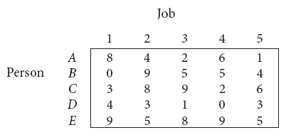
5.
Solve cos2 x \(\frac{dy}{dx}\) + y = tan x
6.
The marginal revenue ‘y’ of output ‘q’ is given by the equation \(\frac { dy }{ dq } =\frac { { q }^{ 2 }+{ 3 }y^{ 2 } }{ 2qy } \). Find the total Revenue function when output is 1 unit and Revenue is Rs. 5.
7.
Compute the average seasonal movement for the following series
| Year | Quarterly Production | |||
| I | II | III | IV | |
| 2002 | 3.5 | 3.8 | 3.7 | 3.5 |
| 2003 | 3.6 | 4.2 | 3.4 | 4.1 |
| 2004 | 3.4 | 3.9 | 3.7 | 4.2 |
| 2005 | 4.2 | 4.5 | 3.8 | 4.4 |
| 2006 | 3.9 | 4.4 | 4.2 | 4.6 |
8.
9.
Construct the Laspeyre’s, Paasche’s and Fisher’s price index number for the following data. Comment on the result.
| Commodities | Base Year | Current Year | ||
| Price | Quantity | Price | Quantity | |
| Rice | 15 | 5 | 16 | 8 |
| Wheat | 10 | 6 | 18 | 9 |
| Rent | 8 | 7 | 15 | 8 |
| Fuel | 9 | 5 | 12 | 6 |
| Transport | 11 | 4 | 11 | 7 |
| Miscellaneous | 16 | 6 | 15 | 10 |
10.
Evaluate the integral as the limit of a sum: \(\int _{ 1 }^{ 2 }{ (2x+1) } dx\)
11.
Evaluate the integral as the limit of a sum: \(\int _{ 0 }^{ 1 }{ x } dx\)
12.
A machine produces a component of a product with a standard deviation of 1.6 cm in length. A random sample of 64 componentsvwas selected from the output and this sample has a mean length of 90 cm. The customer will reject the part if it is either less than 88 cm or more than 92 cm. Does the 95% confidence interval for the true mean length of all the components produced ensure acceptance by the customer?
13.
If 5% of the items produced turn out to be defective, then find out the probability that out of 20 items selected at random there are
(i) exactly three defectives
(ii) atleast two defectives
(iii) exactly 4 defectives
(iv) find the mean and variance
14.
If the probability that an individual suffers a bad reaction from injection of a given serum is 0.001, determines the probability that out of 2,000 individuals
(a) exactly 3, and
(b) more than 2 individuals will suffer a bad reaction.
15.
The demand equation for a product is pd = 20 − 5x and the supply equation is ps = 4x + 8. Determine the consumer’s surplus and producer’s surplus under market equilibrium.
16.
A continuous random variable X has the following probability function
| Value of X = x | 0 | 1 | 2 | 3 | 4 | 5 | 6 | 7 |
| P(x) | 0 | k | 2k | 2k | 3k | k2 | 2k2 | 7k2+k |
(i) Find k
(ii) Ealuate p(x<6), p(x\(\ge \)6) and p(0)
(iii) If P(X\(\le\)x).\(\frac{1}{2}\), then find the minimum value of x.
17.
The elasticity of demand with respect to price p for a commodity is \(\eta _{ d }=\frac { p+2{ p }^{ 2 } }{ 100-p-{ p }^{ 2 } } \).Find demand function where price is Rs. 5 and the demand is 70.
18.
The amount of bread (in hundreds of pounds) x that a certain bakery is able to sell in a day is found to be a numerical valued random phenomenon, with a probability function specified by the probability density function f(x) is given by
\(f(x)=\left\{\begin{array}{l} Ax,for \ 0≤x10 \\ A(20−x),for \ 10 ≤x< 20 \\ 0,\quad \quad \quad otherwise \end{array}\right.\)
(a) Find the value of A.
(b) What is the probability that the number of pounds of bread that will be sold tomorrow is
(i) More than 10 pounds,
(ii) Less than 10 pounds, and
(iii) Between 5 and 15 pounds?
19.
An automobile company uses three types of Steel S1, S2 and S3 for providing three different types of Cars C1, C2 and C3. Steel requirement R (in tonnes) for each type of car and total available steel of all the three types are summarized in the following table.
| Types of Steel | Types of Car | Total Steel available | ||
| C1 | C2 | C3 | ||
| S1 | 3 | 2 | 4 | 28 |
| S2 | 1 | 1 | 2 | 13 |
| S3 | 2 | 2 | 2 | 14 |
Determine the number of Cars of each type which can be produced by Cramer’s rule.
20.
Show that the equations x + y + z = 6, x + 2y + 3z = 14, x + 4y + 7z = 30 are consistent and solve them.
21.
E f (x)= _______.
f(x− h)
f (x)
f(x+ h)
f(x+ 2h)
22.
E ≡ _______.
1 + Δ
1 - Δ
1 + ∇
1 - ∇
23.
The solution for an assignment problem is optimal if _______.
each row and each column has no assignment
each row and each column has atleast one assignment
each row and each column has atmost one assignment
each row and each column has exactly one assignment
24.
25.
The general solution of the differential equation \(\frac{dy}{dx}\) = cos x is ______.
y = sinx + 1
y = sinx - 2
y = cos x + c, c is an arbitrary constant
y = sin x + c, c is an arbitrary constant
26.
27.
The upper control limit for \(\overset {-}{X}\) chart is given by ________.
\(\bar { X } +{ A }_{ 2 }\bar { R } \)
\(\overset { = }{ X } +{ A }_{ 2 }R\)
\(\overset { = }{ X } +{ A }_{ 2 }\bar { R } \)
\(\overset { = }{ X } +{ A }_{ 2 }\overset { = }{ R } \)
28.
The components of a time series which is attached to short term fluctuation is ________.
Secular trend
Seasonal variations
Cyclic variation
Irregular variation
29.
An estimator is said to be ________ if it contains all the information in the data about the parameter it estimates.
efficient
sufficient
unbiased
consistent
30.
31.
The value of \(\int _{ -\frac{\pi}{2}}^{ \frac{\pi}{2}}\) cos x dx is _______.
0
2
1
4
32.
ഽ\(\sqrt { { e }^{ x } } \) dx is _______.
\(\sqrt { { e }^{ x } } +c\)
\(2\sqrt { { e }^{ x } } \) + c
\(\frac12\sqrt { { e }^{ x } } +c\)
\(\frac { 1 }{ 2\sqrt { { e }^{ x } } } +c\)
33.
Let z be a standard normal variable. If the area to the right of z is 0.8413, then the value of z must be: ________.
1.00
-1.00
0.00
-0.41
34.
If X ~ N(9,81) the standard normal variate Z will be ________.
\(Z=\frac { X- 81 }{ 9 } \)
\(Z=\frac { X-9 }{ 81 } \)
\(Z=\frac { X-9 }{ 9 } \)
\(Z=\frac { 9-X }{ 9 } \)
35.
If we have f(x)=2x, 0\(\le\)x\(\le\)1, then f (x) is a ________.
probability distribution
probability density function
distribution function
continuous random variable
36.
A variable that can assume any possible value between two points is called ________.
discrete random variable
continuous random variable
discrete sample space
random variable
37.
The marginal revenue and marginal cost functions of a company are MR = 30 − 6x and MC = −24 + 3x where x is the product, then the profit function is ________.
9x2 + 54x
9x2 − 54x
54x - \(\frac { { 9x }^{ 2 } }{ 2 } \)
54x - \(\frac { { 9x }^{ 2 } }{ 2 } \) + k
38.
Area bounded by the curve y = \(\frac{1}{x}\) between the limits 1 and 2 is ________.
log 2 sq.units
log 5 sq.units
log 3 sq.units
log 4 sq.units
39.
If \(\rho(A) \neq \rho(A, B)\), then the system is _______.
Consistent and has infinitely many solutions
Consistent and has a unique solution
inconsistent
consistent
40.
The rank of the unit matrix of order n is ________.
n −1
n
n +1
n2
41.
Evaluate the following
\(\Gamma \) \(\left( \frac { 9 }{ 2 } \right) \)
42.
Using the following Tippett’s random number table,
| 2952 | 6641 | 3992 | 9792 | 7969 | 5911 | 3170 | 5624 |
| 4167 | 9524 | 1545 | 1396 | 7203 | 5356 | 1300 | 2693 |
| 2670 | 7483 | 3408 | 2762 | 3563 | 1089 | 6913 | 7991 |
| 0560 | 5246 | 1112 | 6107 | 6008 | 8125 | 4233 | 8776 |
| 2754 | 9143 | 1405 | 9025 | 7002 | 6111 | 8816 | 6446 |
Draw a sample of 15 houses from Cauvery Street which has 83 houses in total.
43.
Find the rank of the matrix A =\(\left( \begin{matrix} 1 & -3 \\ 9 & 1 \end{matrix}\begin{matrix} 4 & 7 \\ 2 & 0 \end{matrix} \right) \)
44.
45.
Consider the following pay-off (profit) matrix Action States
| Action | States | |||
| (s1) | (s2) | (s3) | (s4) | |
| A1 | 5 | 10 | 18 | 25 |
| A2 | 8 | 7 | 8 | 23 |
| A3 | 21 | 18 | 12 | 21 |
| A4 | 30 | 22 | 19 | 15 |
Determine best action using maximin principle.
46.
Calculate four-yearly moving averages of number of students studying in a higher secondary school in a particular city from the following data.
| Year | 2001 | 2002 | 2003 | 2004 | 2005 | 2006 | 2007 | 2008 | 2009 |
| Sales | 124 | 120 | 135 | 140 | 145 | 158 | 162 | 170 | 175 |
47.
Form the differential equation that represents all parabolas each of which has a latus rectum 4a and whose axes are parallel to the x axis.
48.
State any three merits of stratified random sampling.
49.
Evaluate \(\int _{ 0 }^{ 1 }{ ({ e }^{ x }-{ 4a }^{ x }+2+\sqrt [ 3 ]{ x } } )dx\)
50.
The probability that a student get the degree is 0.4 Determine the probability that out of 5 students
(i) one will be graduate
(ii) atleast one will be graduate
51.
If f (x) is defined by f(x)=ke-2x, 0\(\le\)x<\(\infty\) is a density function. Determine the constant k and also find mean.
52.
Find the revenue function and the demand function if the marginal revenue for x units is MR = 10 + 3x − x2.
53.
A company receives a shipment of 200 cars every 30 days. From experience it is known that the inventory on hand is related to the number of days. Since the last shipment, I(x)=200 − 0.2x. Find the daily holding cost for maintaining inventory for 30 days if the daily holding cost is Rs. 3.5
1.
\(\Delta =\left| \begin{matrix} 1 & 4 & 3 \\ 2 & -6 & 6 \\ 5 & -2 & 3 \end{matrix} \right| \)
= \(1\left| \begin{matrix} -6 & 6 \\ -2 & 3 \end{matrix} \right| -4\left| \begin{matrix} 2 & 6 \\ 5 & 3 \end{matrix} \right| +3\left| \begin{matrix} 2 & -6 \\ 5 & -2 \end{matrix} \right| \)
= 1(-18 + 12) - 4(6 - 30) +3 (- 4 +30)
= 1(- 6) - 4(- 24) + 3(26)
= - 6 + 96 + 78 = 168 \(\neq \) 0
Since \(\Delta \neq 0\) the system is consistent with unique solution and Cramer's rule can be applied
\(\Delta x=\left| \begin{matrix} 2 & 4 & 3 \\ -3 & -6 & 6 \\ -5 & -2 & 3 \end{matrix} \right| \)
= \(2\left| \begin{matrix} -6 & 6 \\ -2 & 3 \end{matrix} \right| -4\left| \begin{matrix} -3 & 6 \\ -5 & 3 \end{matrix} \right| +3\left| \begin{matrix} -3 & -6 \\ -5 & -2 \end{matrix} \right| \)
= 2 (- 18 + 12) - 4(- 9 +30) + 3(6 -30)
= 2(- 6) - 4(21) + 3(- 24)
= -12-84-72 =-168
\(\Delta y=\left| \begin{matrix} 1 & 2 & 3 \\ 2 & - & 6 \\ 5 & -5 & 3 \end{matrix} \right| =1\left| \begin{matrix} -3 & 6 \\ -5 & 3 \end{matrix} \right| -2\left| \begin{matrix} 2 & 6 \\ 5 & 3 \end{matrix} \right| +3\left| \begin{matrix} 2 & -3 \\ 5 & -5 \end{matrix} \right| \)
= 1 (-9+30)-2(6-30)+3(- 10+ 15)
= 1(21) - 2(- 24) + 3(5)
= 21 + 48 + 15 = 84
\(\Delta z=\left| \begin{matrix} 1 & 4 & 2 \\ 2 & -6 & -3 \\ 5 & -2 & -5 \end{matrix} \right| \)
= \(1\left| \begin{matrix} -6 & -3 \\ -2 & -5 \end{matrix} \right| -4\left| \begin{matrix} 2 & -3 \\ 5 & -5 \end{matrix} \right| +2\left| \begin{matrix} 2 & -6 \\ 5 & -2 \end{matrix} \right| \)
= 1(30-6)-4(-10+ 15)+2(-4+30)
= 24 - 4(5) + 2(26)
= 24 - 20 + 52 = 56
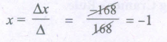
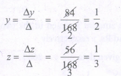
Solution set is \(\left\{ -1,\frac { 1 }{ 2 } ,\frac { 1, }{ 3 } \right\} \)
2.
Since only four values are given,
(E -1)4 u0 = 0
⇒ (E4 - 4E3 + 6E2 - 4E + 1) u0
= u4 - 4 u3 + 6 u2 - 4 u1 + u0
⇒ 385 - 4(u3) + 6(520) - 4 (556) + 560 =0
⇒ 385 - 4u3 + 3120 - 2224 + 560 = 0
⇒ 1841 - 4u3 = 0
⇒ 1841 = 4u3
⇒ u3 = \(\frac{1841}{4}\) = 460.25
∴ u3 = 460.25
3.
Since the pressure required is at the end of the table, we apply Backward interpolation formula. Let temperature be x and the pressure be y.
\({ y }_{ \left( x={ x }_{ 0 }+nh \right) }={ y }_{ 0 }+\frac { n }{ n! } \Delta { y }_{ 0 }+\frac { n(n-1) }{ 2! } { \Delta }^{ 2 }{ y }_{ 0 }+\frac { n(n-)(n-2) }{ 3! } { \Delta }^{ 3 }{ y }_{ 0 }+...\)
To find y at x = 175
\(\therefore\) xn + nh = 175 , xn = 180, h = 10 \(\Rightarrow\) n = −0.5
| x | y | \(\Delta y\) | \(\Delta ^{ 2 }y\) | \(\Delta ^{ 2 }y\) | \(\Delta ^{ 4 }y\) |
| 140 | 3.685 | ||||
| 1.169 | |||||
| 150 | 4.854 | 0.279 | |||
| 1.448 | 02.047 | ||||
| 160 | 6.032 | 0.326 | 0.002 | ||
| 1.774 | 0.049 | ||||
| 170 | 8.076 | 0.375 | |||
| 2.149 | |||||
| 180 | 10.225 |
\({ y }_{ (x=1750 }=10.225+\left( -0.5 \right) (2.149)+\frac { (-0.5)(0-5) }{ 2! } (0.375)+\frac { (-0.5)(0-5)(1.5) }{ 3! } (0.049)+\frac { (-0-5)(0.5)(1.5)(2.5) }{ 4! } (0.002)\)
= 10.225−1.0745−0.046875−0.0030625 − 0.000078125
= 9.10048438
= 9.1
4.
Here the number of rows and columns are equal.
\(\therefore\) The given assignment problem is balanced.
Now let us find the solution.
Step 1: Select a smallest element in each row and subtract this from all the elements in its row.
The cost matrix of the given assignment problem is
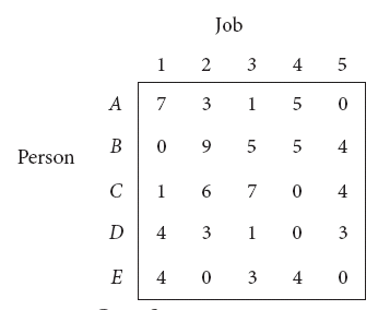
Column 3 contains no zero. Go to Step 2.
Step 2: Select the smallest element in each column and subtract this from all the elements in its column.
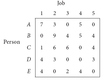
Since each row and column contains atleast one zero, assignments can be made.
Step 3: (Assignment):
Examine the rows with exactly one zero. Row B contains exactly one zero. Mark that zero by \(\square\) (i.e) Person B is assigned to Job 1. Mark other zeros in its column by ×.
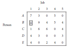
Now, Row C contains exactly one zero. Mark that zero by \(\square\). Mark other zeros in its column by × .
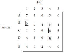
Now, Row D contains exactly one zero. Mark that zero by \(\square\) . Mark other zeros in its column by × .
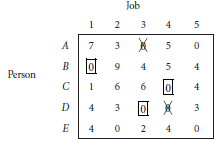
Row E contains more than one zero, now proceed column wise. In column 1, there is an assignment. Go to column 2. There is exactly one zero. Mark that zero by \(\square\) . Mark other zeros in its row by × .
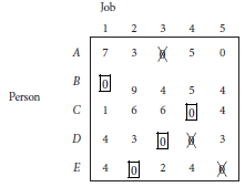
There is an assignment in Column 3 and column 4. Go to Column 5. There is exactly one zero. Mark that zero by \(\square\) . Mark other zeros in its row by × .
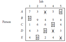
Thus all the five assignments have been made. The Optimal assignment schedule and total cost is
| Person | Job | cost |
| A | 5 | 1 |
| B | 1 | 0 |
| C | 4 | 2 |
| D | 3 | 1 |
| E | 2 | 5 |
| Total cost | 9 | |
The optimal assignment (minimum) cost = Rs. 9
5.
The given equation can be written as \(\frac { dy }{ dx } +\frac { 1 }{ { cos }^{ 2 }x } y=\frac { tanx }{ { cos }^{ 2 }x } \)
\(\frac { dy }{ dx } \) + y sec2x = tan x sec2x
It is of the form \(\frac{dy}{dx}\) + Py + Q
Here P = sec2x,Q = tanx sec2x
ഽPdx = ഽsec2 x dx = tanx
I.F = eഽpdx = etan x
The required solution is y(I.F) = ഽQ(I.F)dx + c
yetan x = ഽtan x sec2xetan xdx + c
Put tan x = t
Then sec2 xdx = dt
∴ yetan x = ഽtet dt + c
= ഽtd(et) + c
= tet − et + c
= tanx etan x−etan x+ c
yetan x = etan x(tan x − 1) + c
6.
Given that \(MR=\frac { dy }{ dq } =\frac { { q }^{ 2 }+{ 3 }y^{ 2 } }{ 2qy } \) (1)
Put y = vq and \(\frac { dy }{ dq } =v+q\frac { dv }{ dq } \) in (1)
Now (1) becomes
\(v+q\frac { dy }{ dq } =\frac { { q }^{ 2 }+{ 3 }v^{ 2 }{ q }^{ 2 } }{ 2yvq } \)
\(=\frac { 1+3{ v }^{ 2 } }{ 2v } \)
\(q\frac { dv }{ dq } =\frac { 1+3{ v }^{ 2 } }{ 2v } -v\)
\(=\frac { 1+3{ v }^{ 2 }-2{ v }^{ 2 } }{ 2v } \)
\(=\frac { { 1+v }^{ 2 } }{ 2v } \)
\(\frac { 2v }{ { 1+v }^{ 2 } } dv=\frac { dq }{ q } \)
On Integration
\(ഽ\frac { 2v }{ { 1+v }^{ 2 } } dv=ഽ\frac { dq }{ q } \)
log (1+ v2) = log q + log c
1+ v2 = cq
Replace \(v=\frac { y }{ q } \)
\(1+\frac { { y }^{ 2 } }{ { q }^{ 2 } } \) = cq
q2 + y2 = c q3 (2)
Given output is 1 unit and revenue is Rs. 5
∴ (2) ⇒ 1 + 25 = c ⇒ c = 26
∴ The total revenue function is q2 + y2 = 26q3
7.
| Year | Quarterly production | |||
| I | II | III | IV | |
| 2002 | 3.5 | 3.8 | 3.7 | 3.5 |
| 2003 | 3.6 | 4.2 | 3.4 | 4.1 |
| 2004 | 3.4 | 3.9 | 3.7 | 4.2 |
| 2005 | 4.2 | 4.5 | 3.8 | 4.4 |
| 2006 | 3.9 | 4.4 | 18.8 | 20.8 |
| Quarterly Total | 18.6 | 20.8 | 18.8 | 20.8 |
| Average | 3.72 | 4.16 | 3.76 | 20.8 |
Grand average = (3.72 + 4.16 + 3.76 + 4.16)/4 = 3.95
Seasonal Index (S.I) for I quarter = (Average of I quarter)/(Grand Average) \(\times\) 100
S.I. for I quarter = 3.72/3.95 \(\times\) 100 = 94.1772
S.I. for II quarter = 4.16/3.95 \(\times\) 100 = 105.3165
S.I. for III quarter = 3.76/3.95 \(\times\) 100 = 95.1899
S.I. for IV quarter = 4.16/3.95 \(\times\) 100 = 105.3165
Thus we obtain the average seasonal movement.
8.
9.
| Commodities | Base Year | Current Year | p0q0 | p0q1 | p1q0 | p1q1 | ||
| Price (p0) |
Quantity (q1) |
Price ((p0)) |
Quantity (q1) |
|||||
| Rice | 15 | 5 | 16 | 8 | 75 | 120 | 80 | 128 |
| Wheat | 10 | 6 | 18 | 9 | 60 | 90 | 108 | 162 |
| Rent | 8 | 7 | 15 | 8 | 56 | 64 | 105 | 120 |
| Fuel | 9 | 5 | 12 | 6 | 45 | 54 | 60 | 72 |
| Transport | 11 | 4 | 11 | 7 | 44 | 77 | 44 | 77 |
| Miscellaneous | 16 | 6 | 15 | 10 | 96 | 160 | 90 | 150 |
| Total | 376 | 565 | 487 | 709 | ||||
Laspeyre’s price index number
\({ P }_{ 01 }^{ L }=\frac { \sum { { p }_{ 1 }{ q }_{ 0 } } }{ \sum { { p }_{ 0 }{ q }_{ 0 } } } \times 100=\frac { 487}{ 376} \times 100=129.5212\)
Paasche’s price index number
\({ P }_{ 01 }^{ P }=\frac { \sum { { p }_{ 1 }{ q }_{ 1 } } }{ \sum { { p }_{ 0 }{ q }_{ 1 } } } \times 100=\frac { 709 }{ 565 } \times 100=125.4867\)
Fisher’s price index number
\({ P }_{ 01 }^{ F }=\sqrt { \frac { \sum { { p }_{ 1 }{ q }_{ 0 } } \times \sum { { p }_{ 1 }{ q }_{ 1 } } }{ \sum { { p }_{ 0 }{ q }_{ 0 } } \times \sum { { p }_{ 0 }{ q }_{ 1 } } } } \times 100=\sqrt { \frac { 487\times 709}{ 376\times 565} } \times 100=127.4879\)
On an average, there is an increase of 29.52%, 25.48% and 27.48% in the price of the commodities by Laspeyre’s, Paasche’s, Fisher’s price index number respectively, when the base year compared with the current year.
10.
\(\int _{ a }^{ b }{ f(x) } =\lim _{ n\rightarrow \infty \\ h\rightarrow 0 }{ \sum _{ r=1 }^{ n }{ h } f(a+rh) } \)
Here a = 1, b = 2, \(h=\frac { b-a }{ n } =\frac { 2-1 }{ n } =\frac { 1 }{ n } \) and f(x) = 2x + 1
f (a + rh) = f\(\left( 1+\frac { r }{ n } \right) \)
= \(2\left( 1+\frac { r }{ n } \right) +1\)
= \(2+\frac { 2r }{ n } +1\)
f (a + rh) = 3 + \(\frac {2r }{ n } \)
\(\int _{ 1 }^{ 2 }{ (x) } dx=\lim _{ n\rightarrow \infty }{ \sum _{ r=1 }^{ n }{ \frac { 1 }{ n } \left( 3+\frac { 2r }{ n } \right) } } \)
\(=\lim _{ n\rightarrow \infty }{ \sum _{ r=1 }^{ n }{ \frac { }{ } \left( \frac{3}{n}+\frac { 2r }{ n } \right) } } \)
=\(\overset { lt }{ n\rightarrow \infty } \left[ \frac { 3 }{ n } \sum _{ r=1 }^{ n }{ 1 } +\frac { 2 }{ { n }^{ 2 } } \sum _{ r=1 }^{ n }{ r } \right] \)
= \(\lim _{ n\leftarrow \infty }{ \left[ \frac { 3 }{ n } n+\frac { 2 }{ { n }^{ 2 } } \frac { n(n+1) }{ 2 } \right] } \)
= \(3+\lim _{ n\rightarrow \infty }{ \left( 1+\frac { 1 }{ n } \right) } \)
\(\int _{ 1 }^{ 2 }{ f(x) } dx\) = 3 +1 = 4
11.
\(\int _{ a }^{ b }{ f(x) } dx=\lim _{ n\rightarrow \infty \\ h\rightarrow 0 }{ \sum _{ r=1 }^{ n }{ h } f(a+rh) } \)
Here a = 0, b = 1, \(h=\frac { b-a }{ n } =\frac { 1-0 }{ n } =\frac { 1 }{ n } \) and f(x) = x
Now f(a+rh) = \(f (0+ \frac{r}{h}) = f (\frac{r}{n}) = r/n\)
On substituting in (1) we have
\(\int _{ 0 }^{ 1 }{ x } dx=\lim _{ n\rightarrow \infty }{ \sum _{ r=1 }^{ n }{ \frac { 1 }{ n } . } \frac { r }{ n } } \)
\(=\lim _{ n\rightarrow \infty }{ \frac { 1 }{ { n }^{ 2 } } \sum _{ r=1 }^{ n }{ r } } \)
\(=\lim _{ n\rightarrow \infty }{ \frac { 1 }{ { n }^{ 2 } } \frac { n(n+1) }{ 2 } } \)
\(=\lim _{ n\rightarrow \infty }{ \frac { 1 }{ { n }^{ 2 } } } .\frac { { n }^{ 2 }\left( 1+\frac { 1 }{ n } \right) }{ 2 } \)
\(=\frac { 1+0 }{ 2 } =\frac { 1 }{ 2 } \)
∴ \(\int _{ 0 }^{ 1 }{ x } dx=\frac { 1 }{ 2 } \)
12.
Here φ is the mean length of the components in the population.
The formula for the confidence interval is
\(\bar{x}-Z_{\alpha / 2} \frac{\sigma}{\sqrt{n}}<\mu<\bar{x}+Z_{\alpha / 2} \frac{\sigma}{\sqrt{n}}\)
\({ Here } \ \sigma=1.6, Z_{\alpha / 2}=1.96, \bar{x}=90 \text { and } \mathrm{n}=64\)
Then \(S.E=\frac { \sigma }{ \sqrt { n } } =\frac { 1.6 }{ \sqrt { 64 } } =0.2\)
Therefore, 90 - (1.96 x 0.2)\(\le φ \le\) 90 + (1.96 x 0.2)
\(\text { i.e. } \ (89.61 \leq \varphi \leq 90.39)\)
This implies that the probability that the true value of the population mean length of the components will fall in this interval (89.61,90.39) at 95% . Hence we concluded that 95% confidence interval ensures acceptance of the component by the consumer.
13.
Given that probability of getting defective item
p = 5% = \(\frac { 5 }{ 100 } \) ⇒ q = 1-p = \(1-\frac { 5 }{ 100 } =\frac { 95 }{ 100 } \)
n = 20
p(x) = \({ n }_{ C_{ x } }{ p }^{ x }{ q }^{ n-x }\), x = 0,1,2....n
(i) P(Exactly 3 defectives)
= \({ 20 }_{ { C }_{ 3 } }\left( \frac { 5 }{ 100 } \right) ^{ 3 }\left( \frac { 95 }{ 100 } \right) ^{ 20-3 }\)
= \(\\ { 20 }_{ { C }_{ 3 } }\)(0.05)3(0.95)17
= \(\\ \frac { 20\times 19\times 18 }{ 3\times 2\times 1 } \) (0.05)3(0.95)5(0.95)5(0.95)5(0.95)2
= (60 x 19) (0.000125)(0.7738)(0.7738)(0.7738)(0.9025)
= 0.059
(ii) P(atleast 2 defectives)
= P(X≥2) =1-P(X<2)
= 1-[P(X=0) + P(X=1)]
= 1-[\(\\ { 20 }_{ { C }_{ 0 } }\)(0.05)0(0.95)20 + \(\\ { 20 }_{ { C }_{ 1 } }\)(0.05)1(0.95)19]
= 1 - [(0.95)20 + 20 (0.05) (0.95)19]
= 1 - [0.3585 + (0.3774)]
= 1 - [0.7359] = 0.2641.
(iii) P (exactly 4 defectives)
P(X = 4) = \(\\ { 20 }_{ { C }_{ 4 } }\) (0.05)4(0.95)16
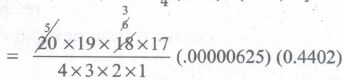
= (15 x 17 x 19) (0.00000625) (0.4402)
= 0.0133
(iv) Find the mean and variance
Mean = np =\(20\times \frac { 5 }{ 100 } =\frac { 100 }{ 100 } \) = 1
Variance =npq = \(20\times \frac { 5 }{ 100 } =\frac { 95 }{ 100 } \) = 0.95
14.
Consider a 2,000 individuals getting injection of a given serum , n = 2000
Let X be the number of individuals suffering a bad reaction.
Let p be the probability that an individual suffers a bad reaction = 0.001
and q = 1– p = 1– 0.001 = 0.999
Since n is large and p is small, Binomial Distribtuion approximated to poisson distribution
So, λ = np = 2000 × 0.001 = 2
(i) Probability out of 2000, exactly 3 will suffer a bad reaction is
\(P(X=3)=\frac { { e }^{ -\lambda }{ \lambda }^{ x } }{ x! } =\frac { { e }^{ -2 }{ 2 }^{ 3 } }{ 3! } =0.1804\)
(ii) Probability out of 2000, more than 2 individuals will suffer a bad reaction
= P(X > 2)
1-[P(X\(\le\)2)]
= 1 – [P(x = 0) + P(x = 1) + P(x = 2)]
\(=1-\left[ \frac { { e }^{ -2 }{ 2 }^{ 0 } }{ 0! } +\frac { { e }^{ -2 }{ 2 }^{ 1 } }{ 1! } +\frac { { e }^{ -2 }{ 2 }^{ 2 } }{ 2! } \right] \)
\(=1-{ e }^{ 2 }\left( \frac { { 2 }^{ 0 } }{ 0! } +\frac { { 2 }^{ 1 } }{ 1! } +\frac { { 2 }^{ 2 } }{ 2! } \right) \)
= 0.323
15.
Given demand function Pd = 20 - 5x and
Supply function Ps = 4x + 8
Under market equilibrium ps = Pd
⇒ 20-5x = 4x+8
⇒ 20-8 = 4x+5x
⇒ 12 = 9x
\(\Rightarrow x=\frac{\not 12}{\not 9}=\frac{4}{3}\)
When \({ x }_{ 0 }=\frac { 4 }{ 3 } ,{ p }_{ 0 }=20-5\left( \frac { 4 }{ 3 } \right) =20-\frac { 20 }{ 3 } \)
\(=\frac { 60-20 }{ 3 } =\frac { 40 }{ 3 } \)
\(\therefore { p }_{ 0 }{ x }_{ 0 }=\frac { 40 }{ 3 } \times \frac { 4 }{ 3 } =\frac { 160 }{ 9 } \)
Consumer Surplus (CS)
\(=\int _{ 0 }^{ x }{ f(x)dx } -{ p }_{ 0 }{ x }_{ 0 }\)
\(=\int _{ 0 }^{ \frac { 4 }{ 3 } }{ (20-5x)dx } \)
\(={ \left[ 20x-\frac { { 5x }^{ 2 } }{ 2 } \right] }_{ 0 }^{ \frac { 4 }{ 3 } }-\frac { 160 }{ 9 } \)
\(=20\left( \frac { 4 }{ 3 } \right) -\frac { 5 }{ 2 } \left( \frac { 16 }{ 9 } \right) -\frac { 160 }{ 9 } \)
\(=\frac { 80 }{ 3 } -\frac { 40 }{ 9 } -\frac { 160 }{ 9 } \)
\(=\frac { 240-40-160 }{ 9 } =\frac { 40 }{ 9 } \)
\(\therefore CS=\frac { 40 }{ 9 }\)units
Producer's Surplus
\((PS)={ p }_{ 0 }{ x }_{ 0 }-\int _{ 0 }^{ x }{ g(x)dx } \)
\(=\frac { 160 }{ 9 } -\int _{ 0 }^{ \frac { 4 }{ 3 } }{ (4x+8)dx } \)
\(=\frac { 160 }{ 9 } -{ \left[ \frac { { 4x }^{ 2 } }{ 2 } +8x \right] }_{ 0 }^{ \frac { 4 }{ 3 } }\)
\(=\frac { 160 }{ 9 } -\left( 2\left( \frac { 16 }{ 9 } \right) +8\left( \frac { 4 }{ 3 } \right) \right) \)
\(=\frac { 160 }{ 9 } -\left( \frac { 32 }{ 9 } +\frac { 32 }{ 3 } \right) \)
\(=\frac { 160 }{ 9 } -\frac { 32 }{ 9 } -\frac { 32 }{ 3 } \)
\(PS=\frac { 160-32-96 }{ 9 } =\frac { 32 }{ 9 } \)units
16.
Given probability function is
| Value of X = x | 0 | 1 | 2 | 3 | 4 | 5 | 6 | 7 |
| P(x) | 0 | k | 2k | 2k | 3k | k2 | 2k2 | 7k2+k |
i) Since the given function is a probability function, each ρi>0 and Σρi=1
⇒ 0+k+2k+2k+3k+k2+2k2+7k2+k = 1
⇒ 10k2+9k = 1
⇒10k2+9k-1 = 0
on factoring we get
(k+1)(10k-1) = 0
⇒k = -1 or k = \(\frac{1}{10}\)
k = -1 is not possible [each ρi>0]
we get k = \(\frac{1}{10}\)
ii) P(X<6) = P(X = 0)+P(X = 1)+P(X=2+P(X=3)+P(X=4)+P(X=5)
P(X<6) = 0 + k + 2k + 2k + 3k + k2
= 8k+k2
= \(8\left( \frac { 1 }{ 10 } \right) { \left( \frac { 1 }{ 10 } \right) }^{ 2 }\)
\(=\frac { 8 }{ 10 } +\frac { 1 }{ 100 } =\frac { 80+1 }{ 100 } =\frac { 81 }{ 100 } \)
\(\therefore P(X<6)=\frac { 81 }{ 100 } \)
Now P(X≥6) = P(X=6)+P(X=7)
= 2k2+7k2+k
= 9k2+k
\(=9{ \left( \frac { 1 }{ 10 } \right) }^{ 2 }+\frac { 1 }{ 10 } \)
\(=\frac { 9 }{ 100 } +\frac { 1 }{ 10 } =\frac { 9+10 }{ 100 } =\frac { 19 }{ 100 } \)
\(\therefore P(X\ge 6)=\frac { 19 }{ 100 } \)
And P(0X<5) = P(X = 1)+P(X = 2)+P(X = 3)+P(X = 4)
= k+2k+2k+3k
\(8k=8\left( \frac { 1 }{ 10 } \right) =\frac { 8 }{ 10 } \)
\( \therefore P(0\))
iii) Given P(X ≤ x) ≥ \(\frac{1}{2}\)
⇒P(X = 0)+P(X = 1)+P(X = 2)+P(X = 3)+P(X = 4)
= 0+k+2k+2k+3k
\(=8k=8\left( \frac { 1 }{ 10 } \right) =\frac { 8 }{ 10 } =\frac { 4 }{ 5 } >\frac { 1 }{ 2 } \)
\(\therefore P(X\le 4)\frac { 1 }{ 2 } \le x=4\)
∴ The minimum value of x is 4.
17.
\(\eta _{ d }=\frac { p+2{ p }^{ 2 } }{ 100-p-{ p }^{ 2 } } \)
\(\frac { -p }{ x } \frac { dx }{ dp } =\frac { p(2p+1) }{ 100-p-{ p }^{ 2 } } \)
\(\frac { -dx }{ x } =\frac { -(2p+1) }{ { p }^{ 2 }+p-100 } dp\)
\(\int { \frac { dx }{ x } } =\int { \frac { 2p+1 }{ { p }^{ 2 }+p-100 } } dp\)
log x = log(p2 + p = 100) + log k
ஃ x = k(p2 + p −100)
When x = 70, p = 5,
70 = k(25 + 5 − 100)
⇒ k = –1
Hence x = 100 − p − p2
R = px
Revenue = p(100 – p – p2)
18.
(a) We know that
\(\int _{ -\infty }^{ \infty }{ f(x) } dx=1\)
\(\int _{ 0 }^{ 10 }{ Axdx } +\int _{ 10 }^{ 20 }{ A(20-x)dx=1 } \)
\(A\left\{ { \left[ \frac { { x }^{ 2 } }{ 2 } \right] }_{ 0 }^{ 10 }+{ \left[ 20x-\frac { { x }^{ 2 } }{ 2 } \right] }_{ 10 }^{ 20 } \right\} =1\)
A[(50-0)+(400-200)-(200-50)] = 1
\(A=\frac{1}{100}\)
(b) (i) The probability that the number of pounds of bread that will be sold tomorrow is more than 10 pounds is given by
\(P(10\le X\le 20)=\int _{ 10 }^{ 20 }{ \frac { 1 }{ 100 } (20-x) } dx\)
\(=\frac { 1 }{ 100 } { \left[ 20x-\frac { { x }^{ 2 } }{ 2 } \right] }_{ 10 }^{ 20 }\)
\(=\frac { 1 }{ 100 } [(400-200)-(200-50)]\)
= 0.5
(ii) The probability that the number of pounds of bread that will be sold tomorrow is less than 10 pounds, is given by
\(P(0\le X\le 20)=\int _{ 0 }^{ 10 }{ \frac { 1 }{ 100 } } xdx\)
\(=\frac { 1 }{ 100 } { \left[ \frac { { x }^{ 2 } }{ 2 } \right] }_{ 0 }^{ 10 }\)
\(=\frac { 1 }{ 100 } (50-0)\)
= 0.5
(ii) The probability that the number of pounds of bread that will be sold tomorrow is between 5 and 15 pounds is
\(P(5\le X \le15)=\int _{ 5 }^{ 10 }{ \frac { 1 }{ 100 } xdx } +\int _{ 10 }^{ 15 }{ \frac { 1 }{ 100 } (20-x)dx } \)
\(=\frac { 1 }{ 100 } { \left[ \frac { { x }^{ 2 } }{ 2 } \right] }_{ 5 }^{ 10 }+\frac { 1 }{ 100 } { \left[ 20x-\frac { { x }^{ 2 } }{ 2 } \right] }_{ 10 }^{ 15 }\)
= 0.75
19.
Let ‘x’ be the number of cars of type C1
Let ‘y’ be the number of cars of type C2
Let ‘z’ be the number of cars of type C3
3x + 2y + 4z = 28
x + y + 2z =13
2x + 2y + z =14
Here \({ \triangle }=\left| \begin{matrix} 3 & 2 & 4 \\ 1 & 1 & 2 \\ 2 & 2 & 1 \end{matrix} \right| =-3\neq 0\)
\({ \triangle }_{ x }=\left| \begin{matrix} 28 & 2 & 4 \\ 13 & 1 & 2 \\ 14 & 2 & 1 \end{matrix} \right| =-6\)
\({ \triangle }_{ y }=\left| \begin{matrix} 3 & 28 & 4 \\ 1 & 1 & 2 \\ 2 & 2 & 1 \end{matrix} \right| =-9\)
\({ \triangle }_{ z }=\left| \begin{matrix} 3 & 2 & 28 \\ 1 & 1 & 13 \\ 2 & 2 & 14 \end{matrix} \right| =-12\)
\(\therefore \) By Cramer’s rule
\(x=\frac { { \triangle }x }{ { \triangle } } =\frac { -6 }{ -3 } =2\)
\(y=\frac { { \triangle }y }{ { \triangle } } =\frac { -9 }{ -3 } =3\)
\(z=\frac { { \triangle }z }{ { \triangle } } =\frac { -12 }{ -3 } =4\)
\(\therefore \) The number of cars of each type which can be produced are 2, 3 and 4.
20.
The matrix equation corresponding to the given system is
\(\left( \begin{matrix} 1 & 1 & 1 \\ 1 & 2 & 3 \\ 1 & 4 & 7 \end{matrix} \right) \left( \begin{matrix} X \\ Y \\ Z \end{matrix} \right) =\left( \begin{matrix} 6 \\ 14 \\ 30 \end{matrix} \right) \)
A X = B
| Augmented matrix [A,B] | Elementary Transformation |
| \(\left( \begin{matrix} 1 & 1 & 1 \\ 1 & 2 & 3 \\ 1 & 4 & 7 \end{matrix}\begin{matrix} 6 \\ 14 \\ 30 \end{matrix} \right) \) \(\sim \left( \begin{matrix} 1 & 1 & 1 \\ 0 & 1 & 2 \\ 0 & 2 & 4 \end{matrix}\begin{matrix} 6 \\ 8 \\ 16 \end{matrix} \right) \) \(\sim \left( \begin{matrix} 1 & 1 & 1 \\ 0 & 1 & 2 \\ 0 & 0 & 0 \end{matrix}\begin{matrix} 6 \\ 8 \\ 0 \end{matrix} \right) \) |
\({ R }_{ 2 }\rightarrow { R }_{ 2 }-{ R }_{ 1 }\) \({ R }_{ 3 }\rightarrow { R }_{ 3 }-{ R }_{ 2 }\) \({ R }_{ 3 }\rightarrow { R }_{ 3 }-{ 2R }_{ 2 }\) |
| \(\rho (A)=2,\rho ([A,B])=2\) |
Obviously the last equivalent matrix is in the echelon form. It has two non-zero rows.
\(\rho (A)=2,\rho ([A,B])=2\)
\(\rho (A)=2,\rho ([A,B])=2\)
The given system is equivalent to the matrix equation,
\(\left( \begin{matrix} 1 & 1 & 1 \\ 0 & 1 & 2 \\ 0 & 0 & 0 \end{matrix} \right) \left( \begin{matrix} X \\ Y \\ Z \end{matrix} \right) =\left( \begin{matrix} 6 \\ 8 \\ 0 \end{matrix} \right) \)
x + y + z = 6 (1)
y + 2z = 8 (2)
\((2)\Rightarrow \)Y = 8 - 2Z,
\((2)\Rightarrow \) X = 6 - Y - Z = 6 - (8 - 2z) - Z = z - 2
Let us take z = k,k \(\in \) R, we get x = k − 2, y = 8 − 2k, Thus by giving different values for k we get different solutions.
Hence the given system has infinitely many solutions.
21.
(c)
f(x+ h)
22.
(a)
1 + Δ
23.
(d)
each row and each column has exactly one assignment
24.
(a)
25.
(d)
y = sin x + c, c is an arbitrary constant
26.
(b)
27.
(c)
\(\overset { = }{ X } +{ A }_{ 2 }\bar { R } \)
28.
(d)
Irregular variation
29.
(b)
sufficient
30.
(b)
31.
(b)
2
32.
(b)
\(2\sqrt { { e }^{ x } } \) + c
33.
(b)
-1.00
34.
(c)
\(Z=\frac { X-9 }{ 9 } \)
35.
(b)
probability density function
36.
(b)
continuous random variable
37.
(d)
54x - \(\frac { { 9x }^{ 2 } }{ 2 } \) + k
38.
(a)
log 2 sq.units
39.
(c)
inconsistent
40.
(b)
n
41.
\(\Gamma \left( \frac { 9 }{ 2 } \right) =\frac { 7 }{ 2 } \Gamma \left( \frac { 7 }{ 2 } \right) \)
\(=\frac { 7 }{ 2 } \Gamma \left( \frac { 5 }{ 2 } \right) \)
\(=\frac { 7 }{ 2 } \times \frac { 5 }{ 2 } \times \Gamma \left( \frac { 3 }{ 2 } \right) \)
\(=\frac { 7 }{ 2 } \times \frac { 5 }{ 2 } \times \left( \frac { 3 }{ 2 } \right) \times \Gamma \left( \frac { 1 }{ 2 } \right) \)
\(=\frac { 7 }{ 2 } \times \frac { 5 }{ 2 } \times \frac { 3 }{ 2 } \times \frac { 1 }{ 2 } \sqrt { \pi } \)
\(=\frac { 105 }{ 16 } \sqrt { \pi } \)
42.
There many ways to select 15 random samples from the given Tippet’s random number table. Since the population size is 83(two-digit number). Here the door numbers are assigned from 1 to 83. Assume that at random we first choose 2nd column. So the first sample is 66 and other 14 samples are 74, 52, 39, 15, 34, 11, 14, 13, 27, 61, 79, 72, 35, and 60. If the numbers are above 83, choose the next number ranging from 1 to 83.
| 2952 | 6641 | 3992 | 9792 | 7969 | 5911 | 3170 | 5624 |
| 4167 | 9524 | 1545 | 1396 | 7203 | 5356 | 1300 | 2693 |
| 2670 | 7483 | 3408 | 2762 | 3563 | 1089 | 6913 | 7991 |
| 0560 | 5246 | 1112 | 6107 | 6008 | 8125 | 4233 | 8776 |
| 2754 | 9143 | 1405 | 9025 | 7002 | 6111 | 8816 | 6446 |
43.
Given A =\(\left( \begin{matrix} 1 & -3 \\ 9 & 1 \end{matrix}\begin{matrix} 4 & 7 \\ 2 & 0 \end{matrix} \right) \)
\(\left( \begin{matrix} 1 & -3 \\ 0 & 28 \end{matrix}\begin{matrix} 4 & 0 \\ -34 & -63 \end{matrix} \right) { R }_{ 2 }\rightarrow { R }_{ 2 }-9{ R }_{ 1 }\)
\(-\left( \begin{matrix} 1 & -3 \\ 0 & 0 \end{matrix}\begin{matrix} 4 & 0 \\ \frac { 10 }{ 3 } & -63 \end{matrix} \right) { R }_{ 2 }\rightarrow { R }_{ 2 }+\frac { 28 }{ 3 } .{ R }_{ 1 }\)
The last equivalent matrix is in echelon form and there are 2 non-zero rows
\(\therefore \rho (A)=2\)
44.
45.
| Action | States | Minimum | |||
| (s1) | (s2) | (s3) | (s4) | ||
| A1 | 5 | 10 | 18 | 25 | 5 |
| A2 | 8 | 7 | 8 | 23 | 7 |
| A3 | 21 | 18 | 12 | 21 | 12 |
| A4 | 30 | 22 | 19 | 15 | 15 |
Max (5,7,12,15) = 15 ஃ Action A4 is the best
46.
Computation of four- yearly moving averages.
| Year | Sales | 4-yearly centered moving total | 4-yearly moving Average | 4-yearly centered moving Average |
| 2001 | 124 | --- | -- | -- |
| 2002 | 120 | -- | -- | -- |
| 519 | 129.75 | |||
| 2003 | 135 | -- | 139.37 | |
| 540 | 135 | |||
| 2004 | 140 | -- | 139.75 | |
| 578 | 144.50 | |||
| 2005 | 145 | -- | 147.87 | |
| 605 | 151.25 | |||
| 2006 | 158 | -- | 162.50 | |
| 635 | 158.75 | |||
| 2007 | 162 | -- | 162.50 | |
| 665 | 166.25 | |||
| 2008 | 170 | -- | -- | - |
| 2009 | 175 | -- | -- | - |
47.
Equation of the family of paraboles with latus rectum 4a and whose axes are parallel to the x-axis is (y- k)2 = 4a(x- h)
[Where (h, k) is the centre of the parabola]
Differentiating w.r.t. 'x' we get,
2(y-k)\(\left( \frac { dy }{ dx } \right) \) = 4a(1)
⇒ 2(y-k)\(\left( \frac { dy }{ dx } \right) \) = 4a (1)
Differentiating again w.r.t x we get,
2(y-k)\(\left( \frac { { d }^{ 2 }y }{ dx^{ 2 } } \right) +\left( \frac { dy }{ dx } \right) (2)\frac { dy }{ dx } \) = 0 (Product rule)
(y-k)\(\left( \frac { d^{ 2 }y }{ dx^{ 2 } } \right) +\left( \frac { dy }{ dx } \right) ^{ 2 }\) = 0 [Divided by 2]
y-k= \(\frac { -\left( \frac { dy }{ dx } \right) ^{ 2 } }{ \frac { { d }^{ 2 }y }{ dx^{ 2 } } } \) (2)
Substituting (2) in (1) we get,
2\(\frac { -\left( \frac { dy }{ dx } \right) ^{ 2 } }{ \frac { { d }^{ 2 }y }{ dx^{ 2 } } } \left( \frac { dy }{ dx } \right) \)= 4a
⇒ \(-2\left( \frac { dy }{ dx } \right) ^{ 3 }=4a\left( \frac { d^{ 2 }y }{ dx^{ 2 } } \right) \)
⇒ \(4a\left( \frac { d^{ 2 }y }{ dx^{ 2 } } \right) +\left( \frac { dy }{ dx } \right) ^{ 3 }\)= 0
\(2a\frac { { d }^{ 2 }y }{ { dx }^{ 2 } } +{ \left( \frac { dy }{ dx } \right) }^{ 3 }=0\).
48.
1. It can be kept small in size without losing its accuracy.
2. It is easy to administer, if the population under study is sub-divided.
3. It reduces the time and expenses in dividing the strata into geographical divisions, since the government itself had divided the geographical areas.
49.
\(\int _{ 0 }^{ 1 }{ ({ e }^{ x }-{ 4a }^{ x }+2+\sqrt [ 3 ]{ x } } )dx\)
= \({ \left[ { e }^{ x }-\frac { 4a }{ \log a } +2x+3\frac { { x }^{ \frac { 4 }{ 3 } } }{ 4 } -1 \right] }_{ 0 }^{ 1 }\)
= \(e-\frac { 4a }{ \log a } +2+\frac { 3 }{ 4 } -1+\frac { 4 }{ \log a } \)
= \(e+\frac { 4(1-a) }{ \log a } +\frac { 7 }{ 4 } \)
50.
Probability of getting a degree p = 0.4
∴ q = 1– p
= 1 - 0.4
= 0.6
(i) P (one will be a graduate) = P(X = 1) = 5C1 (0.4)(0.6)4
= 0.2592
(ii) P ( atleast one will be a graduate) = 1–P (none will be a graduate)
= 1-5C0(P0)(Q)5-0
= 1-5C0(0.4)0(0.6)5
= 1-0.0777
= 0.9222
51.
We know that
\(\int _{ -\infty }^{ \infty }{ f(x)dx=1 } \),since f(x) is a density function
\(\int _{ 0 }^{ \infty }{ { ke }^{ -2x } } dx=1\)
\(k\int _{ 0 }^{ \infty }{ { ke }^{ -2x } } dx=1\)
\(k{ \left[ \frac { { e }^{ -2x } }{ -2 } \right] }_{ 0 }^{ \infty }=1\)
⇒ k = 2
\(E(X)=\int _{ -\infty }^{ \infty }{ xf(x)dx } \)
\(=\int _{ 0 }^{ \infty }{ x{ e }^{ -2x } } dx\)
\(=2\int _{ 0 }^{ \infty }{ { xe }^{ -2x }dx } \)
\(=2\left\{ { \left[ \frac { { xe }^{ -2x } }{ -2 } \right] }_{ 0 }^{ \infty }\int _{ 0 }^{ \infty }{ \frac { { e }^{ -2x } }{ -2 } dx } \right\} \)
\((\because \int { udv=uv-\int { udv } } )\)
\(=\int _{ 0 }^{ \infty }{ { e }^{ -2x }dx } \) \(=\frac { 1 }{ 2 } \)
52.
Given
\(MR=10+3x-{ x }^{ 2 }\)
\(\frac { dR }{ dx } =10+3x-{ x }^{ 2 }\)
\(\Rightarrow dR=(10+3x-{ x }^{ 2 })dx\)
\(\Rightarrow \int { dR } =\int { (10+3x-{ x }^{ 2 }) } dx\)
\(\Rightarrow R=10x+\frac { { 3x }^{ 2 } }{ 2 } -\frac { { x }^{ 3 } }{ 3 } +k\)
When x = 0, R = 0 ⇒ k = 0
\(\Rightarrow R=10x+\frac { { 3x }^{ 2 } }{ 2 } -\frac { { x }^{ 2 } }{ 3 } \)
Demand function\(P=\frac { R }{ x } =\frac { 10x+\frac { { 3x }^{ 2 } }{ 2 } -\frac { { x }^{ 3 } }{ 3 } }{ x } \)
P = 10 + \(\frac { { 3x }^{ 2 } }{ 2 } -\frac { { x }^{ 3 } }{ 3 } \)
53.
Here I(x) = 200 – 0.2x
C1 = Rs. 3.5
T = 30
Total inventory carrying cost = C1\(\int _{ 0 }^{ r }{ I(x) } dx=3.5\int _{ 0 }^{ 30 }{ (200-0.2x) } dx\)
= \(3.5{ \left( 200x-\frac { { 0.2x }^{ 2 } }{ 2 } \right) }_{ 0 }^{ 30 }\) = 20,685

12th Standard Syllabus & Materials
12th Standard
TN 12th Computer Applications களப்பெயர் முறைமை (DNS) Sample Question Papers Study Material - QB365 Set A
NEW12th Standard
TN 12th Computer Applications வலையமைப்பு எடுத்துக்காட்டுகள் மற்றும் நெறிமுறைகள் Sample Question Papers Study Material - QB365 Set A
NEW12th Standard
TN 12th Computer Applications கணினி வலையமைப்பு ஓர் அறிமுகம் Sample Question Papers Study Material - QB365 Set A
NEW12th Standard
TN 12th Computer Applications PHP-உடன் MySQL-ஐ இணைத்தல் Sample Question Papers Study Material - QB365 Set A



Tamilnadu Stateboard 12th Standard Subjects

Maths

Chemistry

Physics

Biology

Computer Science
Business Maths and Statistics

Economics

Commerce

Accountancy

History

Computer Applications
Biology
Computer Technology
Computer Applications
Computer Science
Business Maths and Statistics
Commerce
Economics
Maths
Chemistry
Physics
Computer Technology
History
Accountancy

Tamil

English

French
Tamilnadu Stateboard Standards

