100% FREE ACCESS
11th Standard CBSE Syllabus & Materials
11th Standard CBSE
CBSE 11th Economics PART-A - Presentation of Data - New Sample Question Papers Study Material - QB365 Set A
NEW11th Standard CBSE
CBSE 11th Economics PART-A - Organisation of Data - New Sample Question Papers Study Material - QB365 Set A
NEW11th Standard CBSE
CBSE 11th Economics PART-A - Collection of Data - New Sample Question Papers Study Material - QB365 Set A
NEW11th Standard CBSE
CBSE 11th Economics PART-A - Introduction to Economics and Statistics - New Sample Question Papers Study Material - QB365 Set A
NEW11th Standard CBSE
CBSE 11th Business Studies International Trade Sample Question Papers Study Material - QB365 Set A
NEW11th Standard CBSE
CBSE 11th Business Studies Evolution and Fundamentals of Business Sample Question Papers Study Material - QB365 Set A

Published on: 30/09/2019
Organisation of Data
Download CBSE Class 11th Standard CBSE undefined question papers, sample papers, important questions, and previous year solved papers in PDF format. Get free study materials, NCERT solutions, and exam preparation resources for Class 11th Standard CBSE undefined
Questions + Answers key
Take MCQ Biology Test
1.
Differentiate between Individual, discrete and continuous series.
2.
Differentiate between inclusive and exclusive series
3.
What is a variable? Differentiate between discrete and continuous variable.
4.
Explain the steps involved in construction of a discrete series
5.
What is a statistical series? Explain different types of statistical series on the basis of character
6.
Explain important terms related to a frequency distribution.
7.
Explain different ways of classifying data.
8.
Define classification. What are objectives of classification?
9.
Convert the series given below into exclusive series.
| Age | No of Students |
| (x) | (f) |
| 0-9 | 3 |
| 10-19 | 4 |
| 20-29 | 10 |
| 30-39 | 7 |
| 40-49 | 6 |
10.
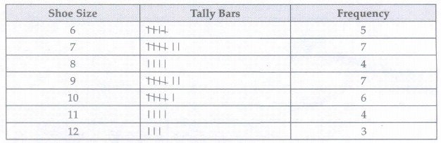
Prepare a discrete frequency distribution of shoe size of your class XI students.
| 7 | 6 | 7 | 8 | 9 | 6 | 7 | 9 | 10 | 12 | 7 | 7 |
| 6 | 8 | 9 | 10 | 11 | 11 | 10 | 9 | 12 | 11 | 10 | 8 |
| 9 | 7 | 6 | 10 | 11 | 12 | 10 | 9 | 9 | 8 | 7 | 6 |
1.
Differentiate between Individual, discrete and continuous series.
| Individual Series | Discrete Series | Continuous Series |
| In individual series, there is only one frequency for each item. | In case of discrete series, there is frequency of more than one for each item. | In case of continuous series, there is frequency of more than one for each item. |
| Individual series has one column and that is of observations. | In discrete there are two columns one for frequency and second for variable. Variable is a number. | In continuous series also, there are two columns as in discrete series but variable is in the form of a class |
| Values are given after a definite break. | Values are given after a definite break. | Values are in the form of groups. |
2.
Differentiate between inclusive and exclusive series
| Basis | Inclusive Series | Exclusive Series |
| Definition | An inclusive series is one in which there is generally a difference between the upper limit of one class interval and the lower limit of the other class interval. | An exclusive series is one in which there is generally no difference between the upper limit of one class interval and the lower limit of the other class interval. |
| Treatment | In inclusive series, value of upper limit of a class is included in that class. | In exclusive series, value of upper limit of a class is not included in that class |
| Utility | It can be used only when value is incomplete number. | It can be used even when value is in decimals or fractions |
| Counting | In inclusive series, counting is not possible without converting it into exclusive series. | Counting can be done in all cases in exclusive series. |
3.
A characteristic or phenomenon which is capable of being measured and changes its value from time to time, place to place or situation to situation is called a variable. In other words, anything which is subject to change in value and can be measured is called a variable. Variable means "which varies". It may vary over time, person to person, place to place etc. for example,Income is a variable as it varies person to person (different people earn different incomes), place to place (salaries vary in India and America) and over time (salaries in 1951 were different from salaries in 2001). Temperature is a variable. It changes over time and also place to place. Height is a variable as it varies person to person and over time.
There are two types of Variable:
Discrete and Continuous
Discrete Variable: A discrete variable is one which increases in jumps or incomplete numbers. For example, there can't be 2.4 workers in a factory. They can be 1, 2, 3, 4 and so on. Similarly, a factory can't have 4.8 or 2/7 machines. It will be incomplete numbers like 1,2,3,4, and soon. Such variable are called discrete variable. Some other examples of discrete variable are number of workers in a factory, number of machines purchased, number of children etc.
Continuous Variable: Those variables which can assume any value in a given range and which increase continuously and not in jumps are called continuous variable. For example, weight of a person can be 45.234 kg, it can take any value within a range. No one gains weight in jumps. It increases in continuity. Other examples are height, income etc.
4.
Following steps are involved in construction of a discrete frequency distribution:
(a) Arrange the series in ascending or descending order: First of all, arrange the raw data in ascending or descending order.
(b) Make as many classes as many are values of variable: Place all values of the variable in the first column of the series beginning with the lowest and giving the highest.
(c) Determine Frequency of each value: To determine frequency of a class, count, how many times a value is repeating itself. For counting, also make a column of tally bars before frequency. A vertical line is put for each repetition and after for five four lines are intersected like this
(d) Place Frequencies:Count the bars. Write it in front of each class in frequency column.
(e) Check Mathematical Accuracy:Total the frequency column to verify if sum total of frequencies is equal to number of total observations.
5.
According to Horace Secrist, "A series as used statistically may be defined as things or attributes of things arranged according to some logical order." According to Prof. Connor, "If two variable quantities can be arranged side by side so that measurable difference in the one corresponds with measurable difference in the other, the result is said to form a statistical series."
On the Basis of Characteristics:
(a) Time Series:
When series of values of some variable which is represented according to successive points in time is called time series. In such a series, data are represented with reference to a time period which can be a year, week, month or day. An example is given below:
Production in a cloth mill
| Year | 2005 | 2006 | 2007 | 2008 | 2009 | 2010 |
| Production(in 000 tonnes) | 15 | 27 | 58 | 72 | 134 | 140 |
or
Rainfall in a week
| DAY | Mon | Tue | Wed | Thu | Fri | Sat | Sun |
| Rainfall in cm |
15 | 27 | 17 | 14 | 54 | 64 | 10 |
(b) Spatial Series: A series of values of some variable which is represented according to area under investigation i.e. geographical division of the universe is called spatial series. An example is given below:
Production of wheat in different states of India in 2010
| States | Punjab | Haryana | Maharashtra | U.P | Bihar | Orissa |
| Production (in 000 tonnes) | 1500 | 2700 | 580 | 720 | 134 | 140 |
(c) Condition Series: A series of values of some variables which is represented according to condition which may be expressed in quantitative terms is called condition series. An example is given below:
| Grade | ||||
| A | B | C | Total | |
| Boys | 13 | 25 | 11 | 49 |
| Girls | 7 | 20 | 6 | 33 |
| Total | 20 | 45 | 17 | 82 |
6.
To understand these terms we are taking two series for reference one is discrete frequency distribution and second is continuous frequency distribution.
Series-1 Discrete Frequency Distribution
| Shoe Size | 7 | 8 | 9 | 10 | 11 | 12 |
| No of Students | 8 | 12 | 20 | 10 | 6 | 4 |
Series-2 Continuous Frequency Distribution
| Marks | 0-10 | 10-20 | 20-30 | 30-40 | 40-50 | 50-60 |
| No of Students | 8 | 12 | 20 | 10 | 6 | 4 |
(a) Frequency: Frequency is the number of times a value repeats itself in the observations. For example when we have written 8 before 7 in series 1, it means 8 students have a shoe size of 7 number in raw data. 12 students have got 8 size, 20 got 9 size and so on. It is applicable to discrete frequency distribution.
(b) Class Frequency: Frequency of a class instead of specific observation is called class frequency. It shows how many items have a value in that class interval. For example, when we have written 10 in column of number of students in front of 30-40, it means 10 students have got marks equal to or more than 30 but less than 40.
(c) Class: It refers to decided group of magnitudes. For example, 0-10 in series 2. It may be 0-9, 10-19 or 4.5 - 8.5 and so on.
(d) Upper and Lower limits of the Class: Lower limit is the lower magnitude of the class and upper limit is the upper magnitude of class. For example in class 0-10, 10 is the lower limit and 10 is the upper limit.
(e) Total Frequency: It is the sum total of frequencies of all classes. It must be equal to total number of observations.
(f)Frequency Distribution: When observations are distributed over several values, it is termed as frequency distribution. For example, in above examples, I series is an example of discrete frequency distribution of shoe size of students. Series 2 is a continuous frequency distribution of marks obtained by students.
(g) Class Interval: Class Interval refers to the magnitude spread between the lower and upper class limit. In other words, it is span or width of the class. It can be obtained by deducting lower limit from upper limit. It is applicable to continuous series only. In series two, class interval is 10 (10-0=10) for first class and for other classes as well. But it is not necessary that all classes should have same class interval. Depending on the purpose, unequal class intervals for different classes can also be used. For example:
| Pocket Expenses | Frequency |
| 0-10 | 2 |
| 10-30 | 9 |
| 30-100 | 3 |
| 100-500 | 5 |
| 500-1000 | 4 |
| 1000-2000 | 2 |
(h) Mid Value: It is the average of lower limit and upper limit. It can be obtained by dividing the sum of lower limit and upper limit by 2. For example, in series 2 given above, we can find mid values as follows:
| Daily Income | No of families | Mid Value |
| 0-100 | 5 | 50 |
| 100-200 | 9 | 150 |
| 200-300 | 12 | 250 |
| 300-400 | 2 | 350 |
| 500 -600 | 2 | 450 |
(i) Discrete Series: A series which represents a discrete variable is called discrete series. For example, series -1 of shoe size is a discrete series.
(j) Continuous Series: A series which represents continuous variable is called a continuous series. For example, in series 2, the distribution of marks amongst students is a continuous series.
7.
Generally, data are classified on the basis of the following four bases:
Geographical Classification:
In geographical classification, data are classified on the basis of geographical or locational differences - such as cities, districts, or villages - between various elements of the data set. The following is an example of a geographical distribution. (Figures are hypothetical)
| States of India | Punjab | Haryana | J & K | Bihar | Orissa | M.P. |
| Poverty (%) |
12 | 10 | 3.5 | 39 | 38 | 34 |
Chronological Classification:
When data are classified on the basis of time, the classification is known as chronological classification. Such classifications are also called time series because data are usually listed in chronological order starting with the earliest period. The following is an example of a Chronological distribution. (Figures are hypothetical)
| Year | 1951 | 1961 | 1971 | 1981 | 1991 | 2001 |
| Poverty (%) | 52 | 50 | 47 | 38 | 36 | 26 |
Another example can be:
| Month | Family expenditure per member |
| January | 2000 |
| February | 3000 |
| March | 1000 |
| April | 1200 |
| May | 2300 |
| June | 1400 |
| July | 1100 |
| August | 4300 |
| September | 900 |
| October | 1900 |
| November | 2100 |
| December | 3100 |
Qualitative Classification:
In qualitative classification, data are classified on the basis of descriptive characteristics or on the basis of attributes like sex, literacy, region, caste, or education, which cannot be quantified. This is done in two ways:
Simple classification:
In this type of classification, each class is subdivided into two sub-classes and only one attribute is studied, for example male and female; blind and not blind, educated and uneducated; and so on.
Manifold classification: In this type of classification, a class is subdivided into more than two subclasses which may be sub-divided further. An example is given below:
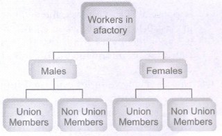
Quantitative Classification: In this classification, data are classified on the basis of characteristics which can be measured such as height, weight, income, expenditure, production, or sales. An example is given below:
| Salary Per Month | No. of workers |
| 0-10000 | 40 |
| 10,000-20,000 | 10 |
| ·20000-30000 | 13 |
| 30000-40000 | 8 |
| 40,000-50,000 | 12 |
| 50,000 and above | 7 |
8.
A classification is an ordered set of related categories used to group data according to its similarities. It consists of codes and descriptors and allows survey responses to be put into meaningful categories in order to produce useful data. Its objectives are as follows:
1. Organized data are attractive and impressive.
2. These are simple and easily understandable.
3. Organization of data is useful in Comparison
4. It saves time effort and energy by simplifying data.
9.
The difference between upper limit and lower limit of two successive classes is1.
Divide one by two.
We get 0.5
Add 0.5 in upper limit of all classes and deduct it from lower limit of all classes. On doing so we get new class intervals as follows:
| Age | No of Students |
| (X) | (f) |
| - 0.5 -9.5 | 3 |
| 9.5 -19.5 | 4 |
| 19.5 - 29.5 | 10 |
| 29.5 - 39.5 | 7 |
| 39.5 - 49.5 | 63 |
10.

11th Standard CBSE Syllabus & Materials
11th Standard CBSE
CBSE 11th Business Studies Forms of Business Organisation Sample Question Papers Study Material - QB365 Set A
NEW11th Standard CBSE
CBSE 11th Business Studies Business, Trade and Commerce Sample Question Papers Study Material - QB365 Set A
NEW11th Standard CBSE
CBSE 11th Physics Waves Sample Question Papers Study Material - QB365 Set A
NEW11th Standard CBSE
CBSE 11th Physics Kinetic Theory Sample Question Papers Study Material - QB365 Set A



CBSE 11th Standard CBSE Subjects
CBSE Standards