100% FREE ACCESS
11th Standard CBSE Syllabus & Materials
11th Standard CBSE
CBSE 11th Economics PART-A - Presentation of Data - New Sample Question Papers Study Material - QB365 Set A
NEW11th Standard CBSE
CBSE 11th Economics PART-A - Organisation of Data - New Sample Question Papers Study Material - QB365 Set A
NEW11th Standard CBSE
CBSE 11th Economics PART-A - Collection of Data - New Sample Question Papers Study Material - QB365 Set A
NEW11th Standard CBSE
CBSE 11th Economics PART-A - Introduction to Economics and Statistics - New Sample Question Papers Study Material - QB365 Set A
NEW11th Standard CBSE
CBSE 11th Business Studies International Trade Sample Question Papers Study Material - QB365 Set A
NEW11th Standard CBSE
CBSE 11th Business Studies Evolution and Fundamentals of Business Sample Question Papers Study Material - QB365 Set A

Published on: 16/12/2019
Production
Download CBSE Class 11th Standard CBSE undefined question papers, sample papers, important questions, and previous year solved papers in PDF format. Get free study materials, NCERT solutions, and exam preparation resources for Class 11th Standard CBSE undefined
Questions + Answers key
Take MCQ Biology Test
1.
Define the law of variable proportions.
2.
How does fall in marginal production affect total output?
3.
What is the law of variable proportions?
4.
What is the average product of an input?
5.
What is the total product of an input?
6.
Complete the following table.
| Units of labour | 0 | 1 | 2 | 3 | 4 | 5 |
| Total product | - | - | - | - | - | - |
| Average product | - | - | - | - | - | - |
| Marginal product | 0 | 10 | 12 | 14 | 14 | 12 |
7.
Explain the relationship between Total Product, Average Product and Marginal Product.
8.
Find out the maximum possible output for a firm with zero unit of Land 10 units of K when its production function is Q = SL + 2K
9.
Let the production function of a firm be Q = 2L2K2 . Find out the maximum possible output that the firm can produce with 5 units of Land 2 units of K. What is the maximum possible output that the firm can produce with zero unit of Land 10 units of K?
10.
The following table gives the average product schedule of labour. Find the total product and marginal product schedules. It is given that the total product is zero at zero level of labour employment.
| L | APL |
| 1 | 2 |
| 2 | 3 |
| 3 | 4 |
| 4 | 4.25 |
| 5 | 4 |
| 6 | 3.5 |
11.
Diminishing marginal returns for the first four units of a variable input is exhibited by the total product sequence:
50, 50, 50, 50
50, 110, 180, 260
50, 100, 150, 200
50, 90, 120, 140
12.
Marginal product, mathematically, is the slope of the
Total product curve
Average product curve
Marginal product curve
Implicit product curve
13.
Diminishing returns occur:
When units of a variable input are added to a fixed input and total product falls.
When units of a variable input are added to a fixed input and marginal product falls.
When the size of the plant is increased in the long run.
When the quantity of the fixed input is increased and returns to the variable input falls.
14.
To economists, the main difference between short run and long run is that:
In short run all inputs are fixed, while in long run all inputs are variable.
In short run the firm varies all of its inputs to find the least cost combination of inputs.
In short run, at least one of the firm's input level is fixed.
In long run, the firm is making a constrained decision about how to use existing plant and equipment efficiently.
15.
The marginal, average, and total product curves encountered by the firm producing in the short run exhibit all of the following relationships except:
When total product is rising, average and marginal product may be either rising or falling.
When marginal product is negative, total product and average product are falling.
When average product is at its maximum, marginal product equals average product, and total product is rising.
When marginal product is at a maximum, average product equals marginal product, and total product is rising.
16.
What are the different phases in the Law of Variable Proportions in terms of marginal product? Give reason behind each phase. Use diagram.
17.
Giving reasons, explain the law of variable proportion.
18.
State the different phases of changes in Total Product and Marginal Product in the Law of Variable Proportions. Also show the same in a single diagram
19.
State the behaviour of marginal product in the law of variable proportions. Explain the causes of this behaviour.
1.
()
The law of variable proportion states that as we increase the quantity of only one input, keeping other inputs fixed, the total product increases at an increasing rate in the beginning, then increases at decreasing rate and after a level the output ultimately falls.
2.
()
Fall in marginal product affects the total output in the following two manners:
(i) When marginal product falls, but remains positive, total product increases at a diminishing rate.
(ii) When marginal product falls and become zero, total product falls in its absolute terms.
3.
()
The law of variable proportion states that as we increase the quantity of only one input, keeping other inputs fixed, the total product increases at an increasing rate in the beginning, then increases at decreasing rate and after a level the output ultimately falls.
4.
()
Average Product of an input is per unit product of variable factors. It is calculated by dividing the total Product by the units of variable factor.
Average product = \(\frac { Total\ product }{ Unit\ of\ variable\ Factor } \)
5.
()
.Total product of an input refers to total volume of goods and services produced by a firm with the given inputs during a specified period of time
6.
| Units of labour | 0 | 1 | 2 | 3 | 4 | 5 |
| Total product = \(\sum \)MPL | 0 | 10 | 22 | 36 | 50 | 62 |
|
Average Product = \(\frac { { TP }_{ L } }{ L } \) |
- | 10 | 11 | 12 | 12.5 | 12.4 |
| Marginal product | 0 | 10 | 12 | 14 | 14 | 12 |
7.
(i) In the beginning Total Product, Average Product and Marginal Product all increase, but Marginal Product> Average Product and Total Product > Marginal Product.
(ii) When Marginal Product = 0, Total Product is maximum and constant and Average Product is decreasing.
(iii) Thereafter, both Average Product and Marginal Product continue to decline, but Marginal Product < Average Product and Total Product declines at an absolute term.
(iv) Marginal Product can be zero and negative but Average Product and Total Product can never be zero.
8.
Q = 5L + 2K (Given)
Q = 5 x 0 + 2 x 10
Q = 0 + 20 = 20 units.
So, the maximum possible output (Q) = 20 units
9.
(i) Q = 2L2 K2(Given)
Q = 2 x 52 x 22
Q = 2 x 25 x 4 = 200 units.
So, the maximum possible output (Q) = 200 units.
(ii) Q = 2L2 K2(Given)
Q = 2 x 02 x 102
Q = 2 x 0 x 20 = 0
So, the maximum possible output (Q) = 0 units
10.
| L | APL | TPL = APL X L |
MPL = \(\frac { { \Delta P }_{ L } }{ \Delta L } \) |
| 1 | 2 | 2 | 2 |
| 2 | 3 | 6 | 4 |
| 3 | 4 | 12 | 6 |
| 4 | 4.25 | 17 | 5 |
| 5 | 4 | 20 | 3 |
| 6 | 3.5 | 21 | 1 |
11.
(d)
50, 90, 120, 140
12.
(a)
Total product curve
13.
(b)
When units of a variable input are added to a fixed input and marginal product falls.
14.
(c)
In short run, at least one of the firm's input level is fixed.
15.
(d)
When marginal product is at a maximum, average product equals marginal product, and total product is rising.
16.
The behaviour of Marginal product in the law of variable proportion is as under:
(i) When Marginal product rises (till Point PI), Total product increases at an increasing rate (convex shape) (till point P).
(ii) When Marginal product falls and remains positive (till point B1), total product increases at a diminishing rate (concave shape) (till point A).
(iii) When Marginal Product is zero (at point B1), Total Product is at its maximum and constant (At point B).
(iv) When Marginal product becomes negative (after point B1), total product falls (after point B).
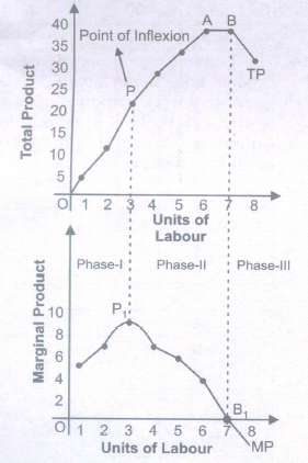
Causes or Reasons of this Behaviour is as Under:
(i) Phase I
(a) Proper utilization of the fixed factor
1. In the initial stage of production, the units of variable input (i.e., labour) is so less that fixed inputs cannot be effectively utilized.
2. Proper utilization of the fixed factor can be attained when more and more units of variable factor (labour units) are applied to the fixed factor (land), the fixed factor will be used intensively and output will increase rapidly.
(b) Specialization and division of labour
1. Initially, there was only one labour working on all the 5 acres of land ploughing, watering, etc.
2. As the number of labour units increases, each worker specialized in a particular activity leads to
specialization of the variable units and this resulted in increased output.
(ii) Phase II
(a) The non-optimal combination of variable factor with the fixed factor
1. When a given quantity of a fixed factor is combined with more and more units of variable factor, the additional units of variable factor will have smaller and smaller quantity of fixed factor to work with them.
2. As many workers share the same fixed factor, the share of each would obviously fall. Therefore, the cooperation of the fixed factor is not available to the same extent. Thus, an increase in the variable factor would add less and less to total output.
(b) Imperfect Substitutes
1. Diminishing return to factor occurs because variable factor and fixed factor are imperfect substitutes to each other.
2. Technically speaking, there is a limit to which variable factor can be applied to fixed factor and that limit depends upon the efficiency of fixed factor. So, variable factor and fixed factor are imperfect substitutes to each other.
(iii) Phase III
(a) Efficiency of Variable Factor Fall
1. In this stage the amount of variable factor becomes excessive relative to the fixed factor. This happens when too many LABOUR are engaged in cultivating on a given piece of land.
2. Instead of helping each other in production they cause overcrowding and chaos and thus hamper each other's work. In such a case, the contribution of additional labour to production is bound to be negative.
3. Thus, the marginal returns become negative and the total returns start diminishing.
(b) Efficiency of Fixed Factor Fall
1. Too much of a variable factors may also lead to the inefficiency of the fixed factor as well. • In case of capital, which is a fixed factor, too much of labour may cause lot of wear and tear of machinery, frequent breakdowns and excessive cost of maintenance. This is bound to affect total production adversely.
2. In such a situation it is advisable to reduce the units of the variable factor than to increase it with a view for getting maximum production.
17.
The behaviour of Marginal product in the law of variable proportion is as under:
(i) When Marginal product rises (till Point PI), Total product increases at an increasing rate (convex shape) (till point P).
(ii) When Marginal product falls and remains positive (till point B1), total product increases at a diminishing rate (concave shape) (till point A).
(iii) When Marginal Product is zero (at point B1), Total Product is at its maximum and constant (At point B).
(iv) When Marginal product becomes negative (after point B1), total product falls (after point B).
Causes or Reasons of this Behaviour is as Under:
(i) Phase I
(a) Proper utilization of the fixed factor
1. In the initial stage of production the units of variable input (i.e., labour) is so less that fixed inputs cannot be effectively utilized.
2. Proper utilization of the fixed factor can be attained when more and more units of variable factor (labour units) are applied to the fixed factor (land), the fixed factor will be used intensively and output will increase rapidly.
(b) Specialization and division of labour
1.Initially there was only one labour working on all the 5 acres of land ploughing, watering, etc.
2. As the number of labour units increases, each worker specialized in a particular activity leads to
specialization of the variable units and this resulted in increased output.
(ii) Phase II
(a) The non-optimal combination of variable factor with the fixed factor
1. When a given quantity of a fixed factor is combined with more and more units of variable factor, the additional units of variable factor will have smaller and smaller quantity of fixed factor to work with them.
2. As many workers share the same fixed factor, the share of each would obviously fall. Therefore, the cooperation of the fixed factor is not available to the same extent. Thus, an increase in the variable factor would add less and less to total output.
(b) Imperfect Substitutes
1. Diminishing return to factor occurs because variable factor and fixed factor are imperfect substitutes to each other.
2. Technically speaking, there is a limit to which variable factor can be applied to fixed factor and that limit depends upon the efficiency of fixed factor. So, variable factor and fixed factor are imperfect substitutes to each other.
(iii) Phase III
(a) Efficiency of Variable Factor Fall
1. In this stage the amount of variable factor becomes excessive relative to the fixed factor. This happens when too many LABOUR are engaged in cultivating on a given piece of land.
2. Instead of helping each other in production they cause overcrowding and chaos and thus hamper each other's work. In such a case, the contribution of additional labour to production is bound to be negative.
3. Thus, the marginal returns become negative and the total returns start diminishing.
(b) Efficiency of Fixed Factor Fall
1. Too much of a variable factors may also lead to the inefficiency of the fixed factor as well. • In case of capital, which is a fixed factor, too much of labour may cause lot of wear and tear of machinery, frequent breakdowns and excessive cost of maintenance. This is bound to affect total production adversely.
2. In such a situation it is advisable to reduce the units of the variable factor than to increase it with a view for getting maximum production.
18.
According to the Law of Variable Proportion when only one input is increased while all other inputs are kept constant, Marginal Product and Total Product behave in the following manner:
(i) When Marginal product rises (till Point PI), Total product increases at an increasing rate (convex shape) (till point P).
(ii) When Marginal product falls and remains positive (Till point B1), total product increases at a diminishing rate (concave shape) (till point A).
(iii) When Marginal Product is zero (at point B1), Total Product is at its maximum and constant (At point B).
(iv) When Marginal product becomes negative (after point B1), total product falls (after point B).
19.
The behaviour of Marginal product in the law of variable proportion is as under:
(i) When Marginal product rises (till Point P1), Total product increases at an increasing rate (convex shape) (till point P).
(ii) When Marginal product falls and remains positive (till point B1), total product increases at a diminishing rate (concave shape) (till point A).
(iii) When Marginal Product is zero (at point B1), Total Product is at its maximum and constant (At point B).
(iv) When Marginal product becomes negative (after point B1), total product falls (after point B).
Causes or Reasons of this Behaviour is as Under:
(i) Phase I
(a) Proper utilization of the fixed factor
1. In the initial stage of production the units of variable input (i.e., labour) is so less that fixed inputs cannot be effectively utilized.
2. Proper utilization of the fixed factor can be attained when more and more units of variable factor (labour units) are applied to the fixed factor (land), the fixed factor will be used intensively and output will increase rapidly.
(b) Specialization and division of labour
1. Initially, there was only one labour working on all the 5 acres of land ploughing, watering, etc.
2. As the number of labour units increases, each worker specialized in a particular activity leads to
specialization of the variable units and this resulted in increased output.
(ii) Phase II
(a) The non-optimal combination of variable factor with the fixed factor
1. When a given quantity of a fixed factor is combined with more and more units of variable factor, the additional units of variable factor will have smaller and smaller quantity of fixed factor to work with them.
2. As many workers share the same fixed factor, the share of each would obviously fall. Therefore, the cooperation of the fixed factor is not available to the same extent. Thus, an increase in the variable factor would add less and less to total output.
(b) Imperfect Substitutes
1. Diminishing return to factor occurs because variable factor and fixed factor are imperfect substitutes to each other.
2. Technically speaking, there is a limit to which variable factor can be applied to fixed factor and that limit depends upon the efficiency of fixed factor. So, variable factor and fixed factor are imperfect substitutes to each other.
(iii) Phase III
(a) Efficiency of Variable Factor Fall
1. In this stage the amount of variable factor becomes excessive relative to the fixed factor. This happens when too many LABOUR are engaged in cultivating on a given piece of land.
2. Instead of helping each other in production they cause overcrowding and chaos and thus hamper each other's work. In such a case, the contribution of additional labour to production is bound to be negative.
3. Thus, the marginal returns become negative and the total returns start diminishing.
(b) Efficiency of Fixed Factor Fall
1. Too much of a variable factors may also lead to the inefficiency of the fixed factor as well. • In case of capital, which is a fixed factor, too much of labour may cause lot of wear and tear of machinery, frequent breakdowns and excessive cost of maintenance. This is bound to affect total production adversely.
2. In such a situation it is advisable to reduce the units of the variable factor than to increase it with a view for getting maximum production.

11th Standard CBSE Syllabus & Materials
11th Standard CBSE
CBSE 11th Business Studies Forms of Business Organisation Sample Question Papers Study Material - QB365 Set A
NEW11th Standard CBSE
CBSE 11th Business Studies Business, Trade and Commerce Sample Question Papers Study Material - QB365 Set A
NEW11th Standard CBSE
CBSE 11th Physics Waves Sample Question Papers Study Material - QB365 Set A
NEW11th Standard CBSE
CBSE 11th Physics Kinetic Theory Sample Question Papers Study Material - QB365 Set A



CBSE 11th Standard CBSE Subjects
CBSE Standards