Chart is a powerful way to convey information to the reader through a pictorial representation. This facility enhances the presentation of data in an effective manner.

(i) Relative cell addressing
(ii) Absolute cell addressing

Frozen columns and rows remain the view during scrooling, whereas other rows and columns gets scrolled

There are two methods to give a more meaningful name to a sheet.
Method 1:
(i) Double-click on a Sheet in which you want rename.
(ii) A small "Rename Sheet" box is appears.
(ii) Type a new name and click "OK" button.
Method 2:
(i) Right-click on a sheet tab and choose Rename Sheet option from the pop-up menu now.
(ii) Now Rename Sheet dialog box appears and type a new name and then click on ok button.

Select continuous: The following steps should be followed to select multiple continuous sheets.
(i) Click on the sheet tab for the first desired sheet.
(ii) Hold down the Shift key and click on the last sheet tab.
non-continous sheets: If you want to select multiple non-continuous sheets the following steps will be followed.
(i) Click on any sheet,
(ii) Hold down the Ctrl key,
(iii) Click another sheet.
Ctrl + Click on any sheet is used to select multiple sheets. Selected sheets tab colour turns into “White”.

Range is the range to which the criteria are to be applied.
Example: Criteria indicates the criteria in the form of a number, an expression or a text string. These criteria determine which cells are counted.
A1:A10 is a cell range containing the numbers 2000 to 2009. Cell B1 contains the number 2006. In cell B2, you enter a formula:
= COUNTIF (A1:A10;2006) - this returns 1

ASIN (Number/Cell Address): This function returns the inverse trigonometric sine of Number that is the angle (in radians) whose sine is Number. The angle returned is in the range – PI/2 to +PI/2. To return the angle in degrees, use the DEGREES function.
Example : = ASIN (0) returns 0. = ASIN (1) returns 1.5707963267949 (PI/2 radians).
= DEGREES (ASIN (0.5)) returns 30. The sine of 30 degrees is 0.5.

(i) To hide or show rows and columns, use the option in the Format menu or the right-click and choose from pop-up menu.
(ii) To hide a row/column, first select the row/column, and then use menu options,
(iii) Format → Row → Hide or Format → Column → Hide to hide row and column respectively,
(iv) The same can be achieved by choosing "Hide" option from the pop-up menu when you right-click the selected row/column.
(v) To show the hidden row/column, choose Format → Row → Show or Format → Column → Show (or)
(vi) Right-click and choose Show from pop-up menu.

A function is a predefined calculation entered in a cell to help to analyze or manipulate data in a spreadsheet. These functions simplify help to create the formulas needed to get the expected results

(i) Relative here means that the reference to this cell address will be changed automatically when you copy the formulae.
(ii) Absolute references are the opposite of relative addressing. A dollar sign is placed before each column name and row number in an absolute reference.

The most commonly used feature input method is built-in functions, the Function Wizard. To open the Function Wizard can be opened through. The menu choose Insert→ Function or using the shortcut key press Ctrl+F2.
(i) Once open, Select a category of functions to shorten the list, then scroll down through the named functions and select the required one.
(ii) When you select a function its description appears on the right-hand side of the dialog. Double-click on the required function.
(iii) The Wizard now displays a textbox where you can enter data manually in text boxes and the result will be displayed in the Result text box
ABS (Number/Cell Address): Number/ Cell Address is the value whose absolute value is to be calculated. The absolute value of a number is its value without +/- sign.
Example : =ABS (-76) returns 76, =ABS (74) returns 7, =ABS (0) returns 0.

Creating and formatting charts :
(i) Select the cells that contain the data that you want to present in your chart.
(ii) Click the Insert → Chart option or click Insert Chart icon on the Standard toolbar.

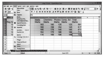
(iii) The Chart Wizard has three main part:
1. List of steps involved in setting up the chart, List of chart types, and The options for each chart type.
2. At any time you can go back to a previous step and change selections.

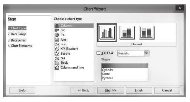
(iv) Choose a Chart type and its option type. Then click Next button.

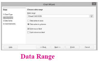
(v) In step 2, Data Range, manually correct any mistakes made in selecting the data. Click one of the options for data series in rows or in columns. Check whether the data range has labels in the first row or in the first column or both. Then click the finish button, or click Next to change some more details of the chart.

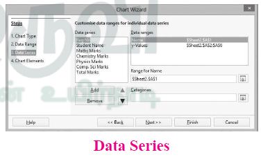
(vi) In the Data Series list box contains a list of all data series in the current chart.
1. To organize the data series, select an entry in the list
2. Click Add to add another data series below the selected entry. The new data series has the same type as the selected entry.
3. Click Remove to remove the selected entry from the Data Series list.
4. Use the Up and Down arrow buttons to move the selected entry in the list up or down. This does not change the order in the data source table, but changes only the arrangement in the chart.
5. Then click Next button.

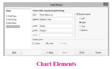
(vii) On the Chart Elements page, chart a title and, if desired, a subtitle. Use a title that draws the viewer's attention to the purpose of the chart: Then click Finish to create chart.

(i) Formatting Data in a cell gives additional effect to the text. Additional effect includes changing the font style, font size, automatic wrapping, bold, underline, italic etc. The data in Calc can be formatted in several ways. Using formatting icons can be used.
(ii) Text formatting : Making the cell contents as bold, italics, underlined, changing font style, size, colour etc., comes under text formatting.
(iii) Number formatting : Number formatting options are used to visually change the format of a numeric content. These formatting changes are appear for visual as, it does not change the original value. For example, To display a number as currency form use Number format: Currency.

In cell A1, type Roll no
In cell B1, type Name
In cell C1, type English
In cell D1, type Tamil
In cell E1, type Maths
In cell F1, type Science
In cell G1, type Social
In cell H1, type Total
In cell 11, type Average.