Total Revenue (TR) :
(i) Total Revenue is the amount of income received by the firm from the sale of its products.
(ii) It is obtained by multiplying the price of the commodity by the number of units sold.
TR = p x Q

(i) Consumer goods are goods which directly satisfy human wants.
(ii) Example: T.V., Furniture, Automobiles, dress, etc

(i) In deductive method we move from general to particular.
(ii) It is also called as analytical (or) abstract method.

(i) Goods are tangible, (eg) car but services are intangible (eg) goodwill.
(ii) Goods can be stored but services cannot be stored.

A cost incurred in the past and cannot be recovered anymore in future, once invested it is treated as drowned or disappeared.

Different types of Elasticity of Demand :
Price Elasticity of Demand
Price elasticity of demand is commonly known as elasticity of demand. This is because price is the most influential factor affecting demand. "Elasticity of demand measures the responsiveness of the quantity demanded to changes in the price".
(1) Price Elasticity of Demand: The price elasticity of demand; commonly known as the elasticity of demand refers to the responsiveness and sensitiveness of demand for a product to the changes in its price. In other words, the price elasticity of demand is equal to
\({ E }_{ p }=\frac { Proportionate \ change \ in \ quantity \ demanded }{ Proportionate \ change \ in \ price } \)
Numerically,
\({ E }_{ p }=\frac { \triangle Q }{ \triangle P } \times \frac { P }{ Q } \)
Where, \(\triangle Q={ Q }_{ 1 }-{ Q }_{ 0 },\triangle P={ P }_{ 1 }-{ P }_{ 0 },Q1\)=New quantity,
\({ Q }_{ 0 }\)=Original quantity, \({ P }_{ 1 }\)=New price, \({ P }_{ 0 }\)=Original price.
(2) Income 'Elasticity of Demand: The income is also a factor that influences the demand for a product. Hence, the degree of responsiveness of a change in demand for a product due to the change in the income is known as income elasticity of demand. , The formula to compute the income elasticity of demand is:
\({ E }_{ Y }=\frac { Proportionate\ change\ in\ quantity\ Demanded\ for\ a\ product }{ Proportionate\ change\ in\ Income } \)
For most of the goods, the income elasticity of demand is greater than one indicating that with the change in income the demand will also change and that too in the same direction, i.e. more income means more demand and vice-versa.
(3) Cross Elasticity of Demand The cross elasticity of demand refers to the percentage change in quantity demanded for one commodity as a result of a small change in the price of another commodity. This type of elasticity usually arises in the case of the interrelated goods such as substitutes and complementary goods. The cross elasticity of demand for goods X and Y can be expressed as:
\({ E }_{ C }=\frac { Proportionate\ change\ in\ Demanded\ of\ commodity\ X }{ Proportionate\ change\ in\ price\ of\ commodity\ Y } \)
(4) Advertising Elasticity of Demand: The responsiveness of the change in demand due to the change in advertising or other promotional expenses, is known as advertising 'elasticity-of demand. It can be expressed as:
\({ E }_{ a }=\frac { Proportionate\ change\ in\ Demand }{ Proportionate\ change\ in\ Advertising\ Expenditure } \)

Marginal Cost:
Marginal cost is defined as the addition made to the total cost by the production of one additional unit of output symbolically.
MC_n = TC_n - TC_n-1 (or) TC_n+1- TC_n
where,
"MC" - Marginal cost.
"TC" - Total cost.
"TC_n" - denotes total cost of "n"^th item.
TC_n-1 - denotes Total cost "n-1"^th item.
TC_n+1 - denotes Total cost of "n+1"^th item.
Marginal cost schedule and MC curve is shown in the following diagram.

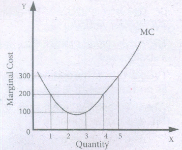
It is to be noted that,
a) MC falls at first due to more efficient use of variable factors.
b) MC curve increases after the lowest point and it slopes upward.
a) MC curve is a "U"- shaped curve.
b) The slope of TC is Me.
If TC = Q3 -18Q2 + 91Q + 12
MC = 3Q2 - 36Q + 91

(i) Man promotes primarily welfare and not wealth.
(ii) The science of economics contains the concerns of ordinary people who are directed by the desired to get maximum monetary benefit.
(iii) Economics is a social science. It studies about I people in the society who influence one another.

(i) Intangible things are not physical objects but exist in connection to other things (eg) goodwill.
(ii) Heterogeneous services vary. A single service gives different experiences (eg) music.
(iii) Inseparable from their makers: Labour and labourer are inseparable.
(iv) Perishable so they cannot be stored in inventories

Short run Average Cost curves:
(i) Average Fixed Cost (AFC)
It refers to the fixed cost per unit of output. It is obtained by dividing the total fixed cost by the quantity of output. AFC = TFC / Q where, AFC denotes average fixed cost, TFC denotes total fixed cost and Q denotes quantity of output. For example, if TFC is 1000 and the quantity of output is 10, the AFC is Rs.100, obtained by dividing Rs.1000 by 10.
Table: Average Fixed Cost

Q (in unit)	TFC (in Rs.)	AFC TFC/Q (in Rs.)
0 1 2 3 4 5	1000 1000 1000 1000 1000 1000	1000/0=\(\infty \) 1000/1=1000 1000/2=500 1000/3=333 1000/4=250 1000/5=200

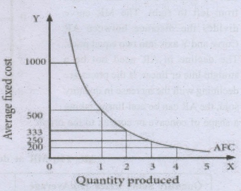
It is to be noted that
(a) AFC declines as output increases, as fixed cost remains constant
(b) AFC curve is a downward sloping throughout its length, never touching X and Y axis. It is asymptotic to both the axes.
(c) The shape of the AFC curve is a rectangular hyperbola.
Average Variable Cost (AVC)
Table: Average Variable Cost

Q(in unit)	TVC (in Rs.)	AVC TVC/Q (in Rs.)
0 1 2 3 4 5	0 200 300 400 600 900	0/0=0 200/1=200 300/2=150 400/3=133 600/4=150 900/5=180

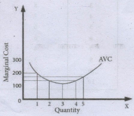
It refers to the total variable cost per unit of output. It is obtained by dividing total variable cost (TVC) by the quantity of output (Q). AVC = TVC / Q where, AVC denotes Average Variable cost, TVC denotes total variable cost and Q denotes quantity of output. For example, When the TVC is Rs. 300 and the quantity produced is 2, the AVC is f RS.150, (AVC = 300/2 = 150)
AVC is shown in table and Diagram
If TVC = Q³ - 18Q² + 9lQ
AVC = Q² -18Q + 91
It is to be noted that
(a) AVC declines initially and then increases with the increase of output.
(b) AVC declines up to a point and moves upwards steeply, due to the law of returns.
(c) AVC curve is a U-shaped curve.
Average Total Cost (ATC) or Average Cost (AC)
It refers to the total cost per unit of output. It can be obtained in two ways.
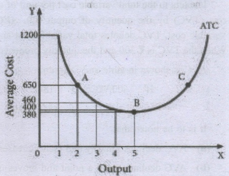
(1) By dividing the firm's total cost (TC) by the quantity of output (Q). ATC = TC / Q. For example, if TC is Rs. 1600 and quantity of output is Q = 4, the Average Total Cost is Rs. 400. (ATC = 1600/4 = 400)
If ATC is Q³ - 18Q² + 91Q +12, then AC = Q² - 18Q +91 + 12/Q
(2) By ATC is derived by adding together Average Fixed Cost (AFC) and Average Variable Cost (AVC) at each level of output ATC = AFC + AVC. For example, when Q = 2, TFC = 1000, TVC = 300; AFC = 500; AVC = 150; ATC = 650. ATC or AC is shown in table and Diagram

 

Q (in unit)	TFC (in Rs.)	TVC (in Rs.)	TC  (in Rs.) TFC+TVC	ATC (TC/Q) (in Rs.)	AFC (in Rs.)	AVC (in Rs.)	ATC (AFC + AVC) (in Rs.)
0 1 2 3 4 5	1000 1000 1000 1000 1000 1000	0 200 300 400 600 900	1000 1200 1300 1400 1600 1900	1000/0=\(\infty \) 1200/1=1200 1300/2=650 1400/3=466 1600/4=400 1900/5=380	0 1000 500 333 250 200	0 200 150 133 150 180	0+0=0 1000+200=1200 500+150=650 333+133=466 250+150=400 200+180=380

It should be noted that 
(a) ATC curve is also a 'U' shaped curve.
(b) Initially the ATC declines, reaches a minimum when the plant is operated optimally, and rises beyond the optimum output.
(c) The 'U' shape of the AC reflects the law of the variable proportions.

Introduction:
The law states that if all other factors are fixed and one input is varied in the short run, the total output will increase at an increasing rate at first, then be constant and finally increase at a declining rate.
Definition:
"As equal increments of one input are added, the inputs of other productive services being held constant, beyond a certain point, the resulting increments of product will decrease (i.e) the MP will diminish". - G. Stigler
Assumptions:
1. Only one factor is variable.
2. All units of the variable factor are homogeneous.
3. The product is measured in physical units.
4. No change in technology.
5. No change in price of the product.

Units of variable factor	Total Product (TPL)	Marginal Product (MPL)	Average Product (APL)	Stages
1 2 3	2 6 12	2 4 6	2 3 4	I
4 5	16 18	4 2	4 3.6	II
6 7	18 16	0 -2	3 2.28	III

x-axis represents labourers. y-axis represents TP_L, MP_L, AP_L

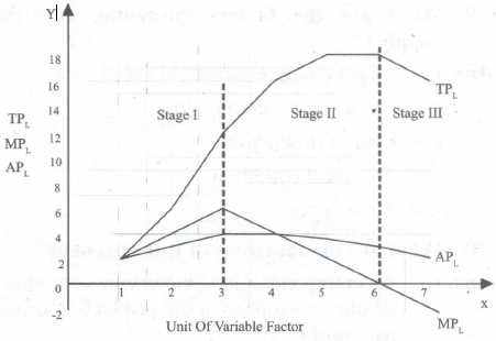
Stages	Total Product (TP)	Marginal Product (MP)	Average Product(AP)
Stage I	It increases at an increasing rate. Then it increases at a decreasing rate. This is the point of inflection.	It increases, reaches maximum and starts to decrease.	It increases, reaches maximum.
Stage II	It continues to increase at a diminishing rate and reaches maximum	lt continues to diminish and becomes zero.	It is equal to MP then begins to diminish.
Stage III	It diminishes.	It becomes negative	It diminishes but always is positive.

Conclusion:
The law of variable proportion helps the producer to decide on the amount of factors to be employed.

Q	Price Rs	TR	AR	MR
1	5	5	5	5
2	5	10	5	5
3	5	15	5	5
4	5	20	5	5
5	5	25	5	5
6	5	30	5	5

\(A R=\frac{T R}{Q}\)

\( M R=T R_{n}-T R_{n-1}\)

Constant AR & MR (fixed price)
When price remains constant, MR is also constant and AR / MR curves coincide.
Declining AR and MR
When a firm sells large quantities at lower prices both AR & MR will fall but the fall in MR will be steeper than the fall in AR.

Q	AR	TR	MR
1	10	10	10
2	9	18	8
3	8	24	6
4	7	28	4
5	6	30	2
6	5	30	0
7	4	28	-2

(i) MR is lower than AR.
(ii) Both AR and MR slope downwards.
(iii) MR divides the distance between AR curve and axis into 2 equal parts.
(iv) The decline in AR need not be a straight line or linear.
(v) If the prices are declining with the increase in quantity sold, the AR can be nonlinear, taking a shape of concave or convex to the origin.