
 100% FREE ACCESS
11th Standard Syllabus & Materials
11th Standard
TN 11th Tamil இயற்கை வேளாண்மை,சுற்றுச்சூழல் -செய்யுள் - மனோன்மணீயம் Important Questions And Answers Study Material - QB365 Set A
NEW11th Standard
TN 11th Tamil என்னுயிர் என்பேன் -துணைப்பாடம் - இசைத்தமிழர் இருவர் Important Questions And Answers Study Material - QB365 Set A
NEW11th Standard
TN 11th Tamil மொழி கலை -செய்யுள் - ஒவ்வொரு புல்லையும் Important Questions And Answers Study Material - QB365 Set A
NEW11th Standard
TN 11th Tamil பீடு பெற நில் - இலக்கணம் - பகுபத உறுப்புகள் Important Questions And Answers Study Material - QB365 Set A
NEW11th Standard
TN 11th Tamil பீடு பெற நில் - துணைப்பாடம் - வாடிவாசல் Important Questions And Answers Study Material - QB365 Set A
NEW11th Standard
TN 11th Tamil பீடு பெற நில் - செய்யுள் - குறுந்தொகை Important Questions And Answers Study Material - QB365 Set A

Published on: 01/07/2021
QB365 provides detailed and simple solution for every Creative Questions in class 11 Economics Subject. It will helps to get more idea about question pattern in every Creative questions with solution.
Download Tamil Nadu 11th Standard Economics question papers, model tests, one-mark questions, important questions, and public exam papers in PDF format. Free study materials and answer keys for TN State Board students.
Questions + Answers key
Take MCQ Economics Test1.
Explain the 'Indifference curve Analysis' with the help of diagrams.
2.
Explain the theory of Consumer's surplus with the help of a table and a diagram.
3.
Explain briefly Levels or degrees of Price Elasticity of Demand?
4.
Explain the indifference curve approach?
5.
Changes in Tastes and fashions the demand for some goods and services is very susceptible to change in tastes and fashions?
1.
INDIFFERENT CURVE ANALYSIS:
Scale of preference:
This theory is also based on scale of preference. A rational consumer usually prefers the combination of goods which gives him maximum level of satisfaction. Thus, the consumer can arrange goods and their combination in order of their satisfaction. Such an arrangement of combination of goods in the order of level of satisfaction is called the "Scale of Preference". Assumptions :
1. The consumer is rational and his aim is to derive maximum satisfaction.
2. Utility cannot be cardinally measured, but can be ranked or compared or ordered by ordinal number such as I, II, III and so on.
3. The Indifference Curve Approach is based on the concept "Diminishing Marginal Rate of Substitution".
4. The consumer is consistent, This assumption is called as the assumption of transitivity. If the consumer prefers combination A to B and B to C, then he should prefer A to C. If A > B and B > C, then A > C.
An Indifference Schedule: An indifference schedule may be defined as a schedule of various combinations of two commodities which will give the same level of satisfaction. In other words, indifference Schedule is a table which shows the different combination of two goods that gives equal satisfaction to the consumer.
Indifference Schedule
| Apple | Orange |
| 1 2 3 4 5 |
20 15 12 10 9 |
Table has five combinations of two commodities. Apple and Orange. Each of these combinations give the consumer the same level of satisfaction without discrimination. In the schedule, the combinations are arranged in such a way that the consumer is indifferent among the combinations. Hence, this schedule is called as, "Indifference Schedule". He will neither be better off nor worse off whichever combination he chooses.
An Indifference Curve
Different combinations of two commodities (as found in Indifference Schedule) can be presented in a diagram. Then consumer gets different points and when such points are connected, a curve is obtained. The said curve is called as "Indifference Curve".
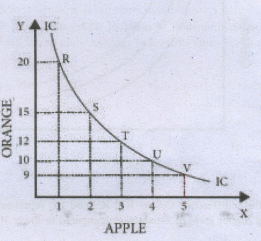
Therefore, an indifference curve is the locus of all combinations of commodities from which the consumer derives the same level of satisfaction. It is also called "Iso-Utility Curve" or Equal Satisfaction Curve". Indifference Curve is illustrated in diagram. X axis represents apple and Y axis represents orange. Point : R' represents combination of 1 apple and 20 oranges, at'S' 2 apples and 15 oranges and at 'T; 3 apples and 12 oranges. Similarly UV points are obtained. These five points give the same level of satisfaction. The consumer will be neither better off nor worse off in choosing anyone of these points. When one joins all these five points (RS, T) U and V one can get the Indifference Curve: IC'.
An Indifference Map :
One can draw several indifference curves each representing an indifference schedule. Hence, an Indifference Map is a family or collection or set of indifference curves corresponding to different levels of satisfaction. The Indifference Map is illustrated in Diagram
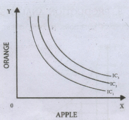
In the diagram, the indifference Curves \({ IC }_{ 1 }\)' \({ IC }_{ 2 }\) and \({ IC }_{ 3 }\) represent the Indifference Map, Upper IC representing higher level of satisfaction compared to lower IC.
2.
Definition: Alfred Marshall defines consumer's surplus as, "the excess of price which a person would be willing to pay a thing rather than go without the thing, over that which he actually does pay is the economic measure of this surplus satisfaction. This may be called consumer's surplus".
Assumption:
(1) Marshall assunied that utility can be measured.
(2) The marginal utilities of money of the consumer remain constant.
(3) There are no substitutes for the commodity in question.
(4) The taste, income and character of the consumer do not change.
(5) Utility of one commodity does not depend upon the other commodities.
Explanation: The concept of consumer's surplus can be explained with the help of an example. Suppose a consumer wants to buy an apple.
He is willing to pay rs.4, rather than go without it and the actual price of the apple is rs.2. Hence the consumer's surplus is rs.2 (rs.4 - rs.2).
Thus, consumer's surplus is the difference between the price that a consumer is willing to pay (potential price) and what he actually pays. Therefore,
Consumer's surplus = What a person is willing to pay - What he actually pays.
OR
Consumer's surplus = Potential price - Actual price.
Mathematically, Consumer's surplus = TU - (P x Q)
where, TU = Total Utility, P = Price and Q = Quantity of the commodity
Assumption:
(1) Marshall assunied that utility can be measured.
(2) The marginal utilities of money of the consumer remain constant.
(3) There are no substitutes for the commodity in question.
(4) The taste, income and character of the consumer do not change.
(5) Utility of one commodity does not depend upon the other commodities.
Explanation:
The concept of consumer's surplus can be explained with the help of an example. Suppose a consumer wants to buy an apple. He is willing to pay Rs 4, rather than go without it and the actual price of the apple is Rs2. Hence the consumer's surplus is Rs2 Rs4 - Rs 2). Thus, consumer's surplus is the difference between the price that a consumer is willing to pay (potential price) and what he actually pays. Therefore,
Consumer's surplus = What a person is willing to pay - What he actually pays.
OR
Consumer's surplus = Potential price - Actual price.
Mathematically,
Consumer's surplus = TU - (P x Q)
where, TU = Total Utility, P = Price and Q = Quantity of the commodity
Consumer's Surplus
| Units of commodity(Apple) | Willingness to pay or potential price(Marginal Utility) | Actual Price | Consumer's Surplus Potential Price Actual Price |
| 1 2 3 4 5 |
6 5 4 3 2 |
2 |
6-2=4 5-2=3 4-2=2 3-2=1 2-2=0 |
| Total | 20 | 10 | 10 |
Where,
TU= Total Utility, P = Price and Q = Quantity of the commodity
The measurement of consumer's surplus is illustrated in the Table.
In the Table the consumer is willing to pay rupees 6, 5, 4, 3 and 2 for purchasing the successive units of apples.
Hence, he is willing to pay (potential Price Total Utility) ~20 for apples. But, he actually pays ~lQ ~2 x 5» for getting 5 apples. Hence,
Consumer's Surplus = Total Utility (Actual Price x units of Commodity)
= TU - (P x Q)
= 20 - (2 x 5)
= 20 - 10 = 10.
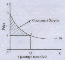
In the diagram, X axis shows the amount demanded and Y axis represents the price.\({ DD }_{ 1 }\) shows the utility which the consumer derives from the purchase of different amounts of commodity.
When price is OP, the amount demanded is OQ. Hence, actual price is OPCQ (OP x OQ). Potential Price (Total Utility) is ODCQ.
Therefore,
Consumer'Surplus = ODCQ - OPCQ
= PDC (the shaded area)
Criticism
(1) Utility cannot be measured, because utility is subjective.
(2) Marginal utility of money does not remain constant.
(3) Potential price is internal, it might be known to the consumer himself.
3.
Definition: The Price Elasticity of Demand is commonly known as the elasticity of demand which refers to the degree of responsiveness of demand to the change in the price of the commodity.
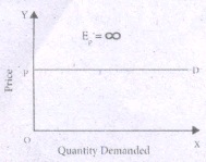
i. Perfectly Elastic Demand (Ep = \(\infty \)):
The demand is said to be perfectly elastic when a slight change in the price of a commodity causes an infinite. change in its quantity demanded. Such as, even a small rise in the price of a commodity can result in greater fall in demand even to zero. In some cases a little fall in the price can result in the increase in demand to infinity. In perfectly elastic demand the demand curve is a horizontal straight line parallel to x axis.
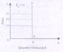
ii. Perfectly Inelastic Demand (Ep = 0)
When there is no change in the product due to the change in the price, then the demand is said to be perfectly inelastic. Here, the demand curve is a vertical straight line which shows that the demand remains unchanged irrespective of change in the price., i.e. quantity OQ remains unchanged at different prices, P1P 2, and P3.
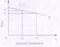
iii. Relatively Elastic Demand: (Ep > 1)
The demand is relatively elastic when the proportionate change in the demand for a commodity is greater than the proportionate change in Its price. Here, the demand curve is gradually sloping which shows that a proportionate change in quantity from 5 to 10 is greater than the proportionate change in the price from 11 to 10. Change in demand is: 10-5/5 x 100 = 100%
Change in price =10%. Hence, it is more elastic demand.
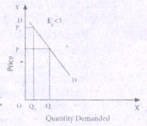
Relatively Inelastic Demand: (Ep < 1)
When the proportionate change in the demand for a product is less than the proportionate change in the price, the demand is said to be relatively inelastic. It is also called as the elasticity less than unity. Here the demand curve is steeply sloping, which shows that the change in the quantity from OQ0 to OQ1 is relatively smaller than the change in the price from OP1 to OP2.
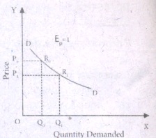
v. Unitary Elastic Demand (Ep = 1):
The demand is unitary elastic when the proportionate change in the price of a product results in the same propionate change in the quantity demand here the shape of the demand curve is a rectangular hyperbola, which shows that area under the curve is equal to one. Here OP0R 0Q 0= OP 1R 1Q 1.
4.
Introduction: J.R.Hicks end R.G.D.Allen refined the Indifference Curve Approach in 1934. Later, in 1939 J.R.Hicks in his book "Value and Capital" gave a final shape to this "Indifference Curve Analysis". This theory is also based on scale of preference.
Assumption:
i. The consumer is rational and his aim is to derive maximum satisfaction.
ii. Utility can be ranked or compared or ordered. by ordinal number such as I, II, III and so on.
iii. The Indifference Curve Approach is based on the concept "Diminishing Marginal Rate of Substitution".
iv. The consumer is consistent. This assumption is called as the assumption of transitivity. If the consumer prefers combination A to B and B to C, then he should prefer A to C. If A>B and B>C, then A>C.
Indifference Schedule:
Indifference Schedule is a table which shows the different combination of two goods that gives equal satisfaction to the consumer.
| Indifference Schedule | |
| Apple | Orange |
| 1 | 20 |
| 2 | 15 |
| 3 | 12 |
| 4 | 10 |
| 5 | 9 |
Table has five combination of two commodities Apple and Orange. This schedule is called as "Indifference Schedule". He will neither be better off nor whose off which ever combination he 4 chooses.
An indifference curve:
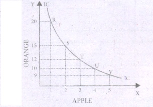
Different combination of two commodities (as found in Indifference Schedule) can be presented in a diagram. Then consumer gets different points and when such points are connected, a curve is obtained. The said curve is called as "Indifference Curve".
An indifference curve is the locus of all combinations of commodities from which the consumer derives the same level of satisfaction. It is also called "Iso-Utility Curve" or Equal Satisfaction Curve".
Explanation:
X axis represents apple and Y axis represents orange. Point 'R' represents combination of 1apple and 20 oranges., at 'S' 2 apples and 15 oranges and at 'T' 3 apples and 12 oranges. Similarly UKV points are obtained. These five points give the same level of satisfaction. The consumer will be neither better off nor worse off ln choosing any one of these points. When one joins all these five points (RS, T) U and V one can get the Indifference Curve 'IC'.
5.
1. Changes in Tastes and Fashions
The demand for some goods and services is very susceptible to changes in tastes and fashions.
2. Changes in Weather: An unusually
dry summer results in a increase in the demand for cool drinks.
3. Taxation and Subsidy
If fresh taxes are levied or the existing rates of taxation on commodities are increased their prices go up. The subsidies will bring down the prices. Therefore taxes reduce demand and subsidies raise demand.
4. Changes in Expectations
Expectations also bring about a change in demand. Expectation of rise in price in future. results in increase in demand.
5. Changes in Savings
Savings and demand are inversely related.
6. State of Trade Activity:
During the periods of boom and prosperity, the demand for all commodities tends to increase. On the contrary, during times of depression there is a general slackening of demand.
7. Advertisement
In advanced capitalistic countries advertising is a powerful instrument increasing the demand in the market.
8. Changes in Income
An increase in family income may increase the demand for durables like video recorders and refrigerators. Equal distribution of income enables poor to get more income. As a result consumption level increases.
9. Change in Population
The demand for goods depends on the size of population. An increase in population tends to increase the demand for goods and a decrease in population.

11th Standard Syllabus & Materials
11th Standard
TN 11th Tamil பீடு பெற நில் - செய்யுள் - காவடிச்சிந்து Important Questions And Answers Study Material - QB365 Set A
NEW11th Standard
TN 11th Tamil பீடு பெற நில் - உரைநடை - மலை இடப்பெயர்கள் : ஓர் ஆய்வு Important Questions And Answers Study Material - QB365 Set A
NEW11th Standard
TN 11th Tamil மாமழை போற்றுதும் - துணைப்பாடம் - யானை டாக்டர் Important Questions And Answers Study Material - QB365 Set A
NEW11th Standard
TN 11th Tamil மாமழை போற்றுதும் - செய்யுள் - ஐங்குறுநூறு Important Questions And Answers Study Material - QB365 Set A



Tamilnadu Stateboard 11th Standard Subjects

Maths

Commerce
Economics

Biology

Business Maths and Statistics

Accountancy

Computer Science

Physics

Chemistry
Maths
Biology
Economics
Physics
Chemistry

History
Business Maths and Statistics

Computer Science
Accountancy

Computer Applications
History
Computer Technology
Commerce
Computer Applications
Computer Technology

Tamil

English

French
Tamilnadu Stateboard Standards



